Generic QC Filters

This section describes how to configure each of the existing QC filters in UFO. All filters can also use the “where” statement to act only on observations meeting certain conditions. By default, each pre and prior filter acts on all the variables marked as observed variables in the ObsSpace, where as post filters act on all simulated variables in the ObsSpace. The filter variables keyword can be used to limit the action of the filter to a subset of these variables or to specific channels, as shown in the examples from the Bounds Check Filter section below.

Bounds Check Filter

This filter rejects observations whose values (ObsValue/ in the ioda files) lie outside specified limits:

- filter: Bounds Check
  filter variables:
  - name: brightnessTemperature
    channels: 4-6
  minvalue: 240.0
  maxvalue: 300.0

In the above example the filter checks if brightness temperature for channels 4, 5 and 6 is outside of the [240, 300] range. Suppose we have the following observation data with 3 locations and 4 channels:

• channel 3: [100, 250, 450]

• channel 4: [250, 260, 270]

• channel 5: [200, 250, 270]

• channel 6: [340, 200, 250]

In this example, all observations from channel 3 will pass QC because the filter isn’t configured to act on this channel. All observations for channel 4 will pass QC because they are within [minvalue, maxvalue]. 1st observation in channel 5, and first and second observations in channel 6 will be rejected.

- filter: Bounds Check
  filter variables:
  - name: airTemperature
  minvalue: 230
- filter: Bounds Check
  filter variables:
  - name: windEastward
  - name: windNorthward
  minvalue: -40
  maxvalue:  40

In the above example two filters are configured, one testing temperature, and the other testing wind components. The first filter would reject all temperature observations that are below 230. The second, all wind component observations whose magnitude is above 40.

In practice, one would be more likely to want to filter out wind component observations based on the value of the wind speed sqrt(windEastward**2 + windNorthward**2). This can be done using the test variables keyword, which rejects observations of a variable if the value of another lies outside specified bounds. The “test variable” does not need to be a simulated or observed variable; in particular, it can be an ObsFunction, i.e. a quantity derived from simulated variables. For example, the following snippet filters out wind component observations if the wind speed is above 40:

- filter: Bounds Check
  filter variables:
  - name: windEastward
  - name: windNorthward
  test variables:
  - name: ObsFunction/Velocity
  maxvalue: 40

If there is only one entry in the test variables list, the same criterion is applied to all filter variables. Otherwise the number of test variables needs to match that of filter variables, and each filter variable is filtered according to the values of the corresponding test variable.

If an observation value happens to be exactly equal to minvalue or maxvalue, the default filter behavior is for that observation to pass QC. (i.e. the passing range of values is inclusive of the endpoints.) This behavior can be changed by setting the min_exclusive and/or max_exclusive parameters to true, in which case observations equal to the specified limits will be rejected. For example, the following filter rejects all temperature observations that are less than or equal to 230:

- filter: Bounds Check
  filter variables:
  - name: airTemperature
  minvalue: 230
  min_exclusive: true

Background Check Filter

This filter checks for bias corrected distance between observation value and model simulated value (\(y-H(x)\)) and rejects observations where the absolute difference is larger than absolute threshold, threshold * \({\sigma}_o\), threshold * \({\sigma}_b\), or threshold * \({\sigma}_e\),where \({\sigma}_o\) is observation error, \({\sigma}_b\) is background error, and \({\sigma}_e\) is the ensemble spread (standard deviation of model equivalents on ensemble members) calculated beforehand by the Ensemble Statistics filter. This filter can also adjust observation error through a constant inflation factor when the filter action is set to inflate error. If no action section is included in the yaml, the filter is set to reject the flagged observations.

- filter: Background Check
  filter variables:
  - name: airTemperature
  threshold: 2.0
  absolute threshold: 1.0
  action:
    name: reject
- filter: Background Check
  filter variables:
  - name: windEastward
  - name: windNorthward
  threshold: 2.0
  where:
  - variable:
      name: MetaData/latitude
    minvalue: -60.0
    maxvalue: 60.0
  action:
    name: inflate error
    inflation factor: 2.0
- filter: Background Check
  filter variables:
  - name: sea_surface_height
  threshold wrt background error: true
  threshold: 2.0

The first filter would flag temperature observations where \(|y-(H(x)+bias)| > \min (\) absolute_threshold, threshold * \({\sigma}_o)\), and then the flagged data are rejected due to the filter action being set to reject.

The second filter would flag wind component observations where \(|y-(H(x)+bias)| >\) threshold * \({\sigma}_o\) and latitude of the observation location are within 60 degree. The flagged data will then be inflated with a factor 2.0.

Please see the Filter Actions section for more detail.

The third filter compares the departure against the background error rather than the observation error. It would flag sea surface height observations where \(|y-(H(x)+bias)| >\) threshold * \({\sigma}_b\), and reject the flagged observations as no filter action is specified. If threshold wrt background error is set to true, then threshold must be set and absolute threshold must not.

There is an option for the background check filter to check for distance between observation value and model simulated value without bias correction (\(y-H(x)\)) when the additional parameter bias correction parameter is set to 1.0 and rejects observations where the absolute difference is larger than absolute threshold or threshold * \({\sigma}_o\) when the filter action is set to reject. If no action section is included in the yaml, the filter is set to reject the flagged observations.

- filter: Background Check
  filter variables:
  - name: brightnessTemperature
    channels: 1-24
  absolute threshold: 3.5
  bias correction parameter: 1.0
  action:
    name: reject

This filter would flag temperature observations where \(|y-H(x)| > \min (\) absolute_threshold, threshold * \({\sigma}_o)\), and then the flagged data are rejected due to filter action is set to reject.

A list of absolute thresholds can be added through the optional input absolute threshold vector in order to set variable-specific thresholds, i.e., different channels in satellite data. Here is an example to conduct Background Check of brightness temperature observations with 13 channels:

- filter: Background Check
  filter variables:
  - name: brightnessTemperature
    channels: 1-13
    threshold: 2.0
    absolute threshold vector: [30.0,30.0,15.0,30.0,15.0,
                                30.0, 5.0,15.0,20.0,20.0,
                                20.0,10.0,10]

It is also possible to compare observations against the ensemble mean of model equivalents and scale the tolerance threshold by the ensemble spread. To this end, these quantities need to be calculated beforehand by the Ensemble Statistics filter, as in the example below:

- filter: Ensemble Statistics
  statistics:
  - MeanHofX                           # Compute ensemble mean
  - HofXStdDev                         # Compute ensemble spread
- filter: Background Check
  test_hofx: MeanHofX                  # Compare with ensemble mean
  threshold wrt ensemble spread: true  # Scale threshold by ensemble spread
  threshold: 2.0
  defer to post: true                  # Ensure the filter is treated as a post-filter

Bayesian Background Check Filter

Similar to the standard Background Check filter, which rejects observations based on the difference between observation value and model simulated value (\(y-H(x)\)), the Bayesian Background Check also takes into account the probability that an observation is “bad”, i.e. “in gross error”. It is expected that the initial Probability of Gross Error (PGE) is set before calling the Bayesian Background Check filter (e.g. using a Variable Assignment filter). In the Bayesian Background Check filter, this initial PGE value determines the weight given to the uniform (“bad”) probability distribution - while (1-PGE) is the weight given to the “good” distribution (a Gaussian in \([y-H(x)]\), with variance \({\sigma}^2\) given by the sum of background uncertainty and observation uncertainty variances). The initial PGE divided by the combined probability distribution, gives the conditional probability that the observation is in gross error. This conditional probability value is the after-check PGE, PGEBd. It is saved in the ObsSpace for optional later use in the buddy check, and observations are also rejected if it exceeds a given threshold. There is also the option of the Bayesian Background Check filter performing a “squared difference” check, to reject observations if \([y-H(x)]^2/{\sigma}^2\) exceeds a threshold.

A useful reference describing the practical implementation of Bayes Theorem for meteorological observations is:

Lorenc, A.C. and Hammon, O. (1988), Objective quality control of observations using Bayesian methods. Theory, and a practical implementation. Q.J.R. Meteorol. Soc., 114: 515-543.

The .yaml file requires that one of the following two filter parameters are set to define the probability distribution for the observation to be bad:

• prob density bad obs (PdBad): In this case the same value is applied to all the observations on which the filter is applied (typically this is set to the inverse of the climatological range e.g. 0.1/K for a domain 273-283 K for some temperature observation).

• prob density bad obs vector name (pdBadObsVectorName): In this case the probability distribution of bad obs is allowed to vary from observation to observation location. The vector should reside in the obspace as part of the MetaData group and be of size nlocations. An application of this is for quality control of land soil moisture observations where the range of soil moisture values can change in different locations according to the soil properties.

The .yaml file can also contain optional filter parameters, which override the default values in ufo/filters/BayesianBackgroundCheck.h and ufo/utils/ProbabilityOfGrossErrorParameters.h:

• PGE threshold (PGECrit, default 0.1): if the adjusted (after-check) PGE exceeds this value, the observation is rejected;

• perform obs minus BG threshold check (PerformSDiffCheck: default true): if true perform an additional squared difference check, that \([y-H(x)]^2/{\sigma}^2\) does not exceed a threshold;

• obs minus BG threshold (SDiffCrit, default 100.0): threshold value for the squared difference check;

• max exponent (ExpArgMax, default 80.0): maximum allowed value of the exponent in the “good” probability distribution;

• obs error multiplier (ObErrMult, default 1.0): weight of observation error in the combined error variance;

• BG error multiplier (BkgErrMult, default 1.0): weight of background error in the combined error variance;

• bg error: constant background error term. If present this will be used instead of the real background errors;

• bg error suffix (BkgErrSuffix, default “_background_error”): suffix which has been appended to variable name for background errors which are to be read in;

• bg error group (BkgErrGroup, default “ObsDiag”): group name which background errors for each variable are stored in;

• save total pd (SaveTotalPd, default false): if true, save the total (combined) probability distribution to the GrossErrorProbabilityTotal group. This is required as an input by the Bayesian Whole Report filter.

• max error variance (ErrVarMax): a maximum value for the error variance. If not set, no maximum is applied.

- filter: Variable Assignment
  assignments:
  - name: GrossErrorProbability/ice_area_fraction
    type: float
    value: 0.04
- filter: Bayesian Background Check
  filter variables:
  - name: ice_area_fraction
  prob density bad obs: 1.0
  PGE threshold: 0.07
  obs minus BG threshold: 100.0

Note that this filter requires the background value (HofX) and background error. Unless a constant background error term ‘bg error’ is provided in the yaml, the latter is accessed from the obs diagnostics - as an interim measure, supplied in a separate .nc4 file (see .yaml snippet below), with variable name e.g. ice_area_fraction_background_error (no group name) to go with ice_area_fraction.

HofX: HofX
obs diagnostics:
  filename: Data/ufo/testinput_tier_1/background_errors_for_bayesianbgcheck_test.nc4

By default, a filter variable is treated as scalar. But for vectors, such as wind, the two components must be specified one after the other in the .yaml, and the first must have the option first_component_of_two set to true.

- filter: Bayesian Background Check
  filter variables:
  - name: windEastward
    options:
        first_component_of_two: true
  - name: windNorthward

Bayesian Background check currently only works for single-level observations, not profiles.

Bayesian Background QC Flags filter

The Bayesian Background QC Flags filter sets diagnostic flags based on values of probability of gross error (PGE). This filter should be invoked after any other filters which modify PGE, such as the Bayesian background check and the buddy check, have been run. If the PGE is larger than a chosen threshold then the observation is rejected by setting flags at the observation location.

The following filter parameters can be set:

• PGE threshold: value of PGE above which an observation is rejected.

• PGE variable name substitutions: a list of pairs of variable names. The PGE of the second variable in each pair is used to set the QC flags of the first variable; by default this happens for wind u and v components.

An example yaml section is as follows:

- filter: Bayesian Background QC Flags
  filter variables: [airTemperature, windEastward, windNorthward]
  PGE threshold: 0.8
  PGE variable name substitutions: {"windEastward", "windNorthward"}

Air temperature QC flags are set if the temperature PGE is greater than 0.8. Due to the use of the variable name substitutions, both eastward and northward wind flags are set if the northward wind PGE is greater than 0.8. This could be useful if the PGE of only one of the wind components has been modified by the QC filters.

Bayesian Whole Report Filter

Synoptic stations typically provide reports at regular intervals. A report is a combination of variables observed by different sensors at a single location. Reports may include some, but not necessarily all, of pressure, temperature, dew point and wind speed and direction.

This filter calculates the probability that a whole report is affected by gross error, through the Bayesian combination of the probability of gross error of individual observations. This is based on the logic that if multiple observations within a report appear dubious based on a Bayesian Background check, it is likely that the whole report is affected by, for example, location error. This filter should be called after the Bayesian Background Check. The probability that whole report is affected by gross error is calculated from all the gross error probability of all the variables in the filter variables list, except where the not_used_in_whole_report option is specified for a given variable.

Once the probability that whole report is affected by gross error has been calculated, it is used to update the probability of gross error for each variable in the filter variables list. Where this updated probability of gross error exceeds the PGE threshold, the observation is flagged. PGE threshold is an optional yaml parameter which applies to the whole filter, and has a default value of 0.1.

Variables can be either scalar or vector (with two Cartesian components, such as the eastward and northward wind components). In the latter case the two components need to be specified one after the other in the filter variables list, with the second component having the second_component_of_two option set to true.

For each variable, the optional parameter probability_density_bad (default value 0.1) is used to set the prior probability density of that variable being “bad”. The filter can also apply a specific prior probability density of bad observations for the following observation types, identified by the integer ID MetaData/ObsType:

• Bogus bogus_probability_density_bad

• Synop (SynopManual, SynopAuto, MetarManual, MetarAuto, SynopMob, SynopBufr, WOW) synop_probability_density_bad

These are both optional parameters. If they are not specified, probability_density_bad is used in their place, as for all other observation types.

For each filter variable, the following groups must be available from the ObsSpace:

• GrossErrorProbability/: the latest value of GrossErrorProbability,

• GrossErrorProbabilityInitial/: the initial value of GrossErrorProbability before updates by any other filter, which can be saved using the Variable Assignment filter,

• GrossErrorProbabilityTotal/: the total (combined) probability distribution, which is optionally saved the Bayesian Background Check filter,

• DiagnosticFlags/BackgroundCheckRejection/: the BackgroundCheckRejection diagnostic flags must be initialized before this filter.

Additionally, the prior probability of gross error applying to the whole report must be available from MetaData/grossErrorProbabilityReport.

Example:

- filter: Bayesian Whole Report
  filter variables:
  - name: pressure_at_model_surface
    options:
      probability_density_bad: 0.1
      bogus_probability_density_bad: 0.1
  - name: air_temperature_at_2m
    options:
      probability_density_bad: 0.1
  - name: windEastward
    options:
      probability_density_bad: 0.1
      synop_probability_density_bad: 0.1
      bogus_probability_density_bad: 0.1
  - name: windNorthward
    options:
      not_used_in_whole_report: true
      second_component_of_two: true
  - name: relativeHumidityAt2M
    options:
      not_used_in_whole_report: true
      probability_density_bad: 0.1
  PGE threshold: 0.15

PreQC Filter

This filter rejects all observations with a PreQC value either greater than a maxvalue or less than a minvalue (both of which default to zero if not provided). The example filter (below) is configured to reject all windSpeed observations whose PreQC value is greater than 3 (and less than zero due to default on minvalue).

- filter: PreQC
  filter variables:
  - name: windSpeed
  maxvalue: 3
  action:
    name: reject

Polygon Check Filter

This pre-filter rejects all observations outside a polygonal region on the sphere.

The Polygon Check filter accepts any valid polygon (concave or convex) and has been tested from 3 up to 12,000 vertices. Vertices are connected via great circle arcs, representing the shortest path on a sphere.

Note

Great circle arcs appear curved on 2D map projections, particularly near the poles. Ensure vertex density is sufficient to maintain the intended shape.

The filter is coordinate-agnostic regarding longitude wrapping. Both commonly-used ranges have been tested:

• \([-180^\circ, 180^\circ]\)

• \([0^\circ, 360^\circ]\)

Specify the polygon using the vertices and a point inside the polygon. Any observations on the opposite side of the polygon from the “inside point” are flagged. What happens to points precisely on a polygon edge will be inconsistent. If you want the edges to be included, then you should enlarge the polygon slightly.

Required input parameters:

vertex longitudes

Longitudes of all vertices of the polygon. Must match latitudes.

vertex latitudes

Latitudes of all vertices of the polygon. Must match longitudes.

inside point longitude

Longitude of a point inside the polygon but not on an edge or vertex.

inside point latitude

Latitude of the same point used in “inside point longitude”

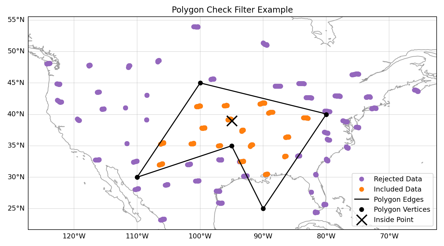
Polygon Filter Example

In this example, we have a concave polygon of 5 vertices over the continental US. We list the vertices as 110 W, 30 N; 100 W, 45 N; 80 W, 40 N; 90 W, 25 N; 95 W, 35 N; and 110 W, 30 N. The first point is the last point, making a closed loop. Our inside point is 95 W, 39 N.

- filter: Polygon Check
  inside point longitude: -95
  inside point latitude: 39
  vertex longitudes: [ -110, -100, -80, -90, -95, -110 ]
  vertex latitudes: [ 30, 45, 40, 25, 35, 30 ]
  action:
    name: reduce obs space

Domain Check Filter

This filter retains all observations selected by the “where” statement and rejects all others. Below, the filter is configured to retain only observations * taken at locations where the sea surface temperature retrieved from the model is between 200 and 300 K (inclusive) * with valid height metadata (not set to “missing value”) * taken by stations with IDs 3, 6 or belonging to the range 11-120 * without valid pressure metadata.

- filter: Domain Check
  where:
  - variable:
      name: GeoVaLs/sea_surface_temperature
    minvalue: 200
    maxvalue: 300
  - variable:
      name: MetaData/height
    value: is_valid
  - variable:
      name: MetaData/stationIdentification
    is_in: 3, 6, 11-120
  - variable:
      name: MetaData/pressure
    value: is_not_valid

BlackList Filter

This filter behaves like the exact opposite of Domain Check: it rejects all observations selected by the “where” statement statement. The status of all others remains the same. Below, the filter is configured to reject observations taken by stations with IDs 1, 7 or belonging to the range 100-199:

- filter: BlackList
  where:
  - variable:
      name: MetaData/stationIdentification
    is_in: 1, 7, 100-199

RejectList Filter

This is an alternative name for the BlackList filter.

AcceptList Filter

This filter sets the QC flag to pass for all observations selected by the “where” statement that have previously been rejected for any reason other than missing data, a pre-processing flag indicating rejection, or failure of the ObsOperator. This is mostly useful in QC procedures where all observations are initially rejected and then those fulfilling certain criteria are accepted, overriding the rejection.

Below, the filter is configured to accept only observations taken by stations with IDs 1, 7 or belonging to the range 100-199 (inclusive):

- filter: RejectList  # initially reject all observations
- filter: AcceptList  # accept back selected observations
  where:
  - variable:
      name: MetaData/stationIdentification
    is_in: 1, 7, 100-199

Perform Action Filter

This filter performs the action specified in the action parameter on observations selected by the “where” statement.

Example 1

Here the filter is configured to inflate errors of all observations from the Southern hemisphere by a factor of two:

- filter: Perform Action
  action:
    name: inflate error
    inflation factor: 2.0
  where:
  - variable: latitude
    maxvalue: 0

Note

Technically, the same result could be obtained by replacing Perform Action in the listing above by RejectList. However, having a RejectList filter that does not actually reject any observations can be confusing.

Example 2

The filter configured in this way behaves like RejectList:

- filter: Perform Action
  action:
    name: reject

Example 3

The filter configured in this way behaves like AcceptList:

- filter: Perform Action
  action:
    name: accept

Thinning Filter

This filter rejects a specified fraction of observations, selected at random. It supports the following YAML parameters:

• amount: the fraction of observations to reject (a number between 0 and 1).

• random seed (optional): an integer used to initialize a random number generator if it has not been initialized yet. If not set, the seed is derived from the calendar time.

Note: because of how this filter is implemented, the fraction of rejected observations may not be exactly equal to amount, especially if the total number of observations is small.

Example:

- filter: Thinning
  amount: 0.75
  random seed: 125

Gaussian Thinning Filter

This filter thins observations by preserving only one observation in each cell of a grid. Cell assignment can be based on an arbitrary combination of:

• horizontal position

• vertical position (in terms of height or pressure)

• time

• category (arbitrary integer associated with each observation).

Selection of the observation to preserve in each cell is based on

• its position in the cell

• optionally, its priority.

The following YAML parameters are supported:

• Horizontal grid:

  • horizontal_mesh: Approximate width (in km) of zonal bands into which the Earth’s surface is split. Thinning in the horizontal direction is disabled if this parameter is negative. Default: approx. 111 km (= 1 deg of latitude).

  • use_reduced_horizontal_grid: True to use a reduced grid, with high-latitude zonal bands split into fewer cells than low-latitude bands to keep cell size nearly uniform. False to use a regular grid, with the same number of cells at all latitudes. Default: true.

  • round_horizontal_bin_count_to_nearest: True to set the number of zonal bands so that the band width is as close as possible to horizontal_mesh, and the number of cells (“bins”) in each zonal band so that the cell width in the zonal direction is as close as possible to that in the meridional direction. False to set the number of zonal bands so that the band width is as small as possible, but no smaller than horizontal_mesh, and the cell width in the zonal direction is as small as possible, but no smaller than in the meridional direction.

    Defaults to false unless the ops_compatibility_mode option is enabled, in which case it’s set to true.

  • partition_longitude_bins_using_mesh: True to calculate partioning of longitude bins explicitly using horizontal mesh distance. By default this option is set to false and calculating the number of longitude bins per latitude bin index involves the integer number of latitude bins. Setting this option to true adopts the Met Office OPS method whereby the integer number of latitude bins is replaced, in the calculation of longitude bins, by the Earth half-circumference divided by the horizontal mesh distance.

    Defaults to false unless the ops_compatibility_mode option is enabled, in which case it’s set to true.

  • define_meridian_20000_km: True to define horizontalMesh with respect to a value for the Earth’s meridian distance (half Earth circumference) of exactly 20000.0 km. By default this option is set to false and the Earth’s meridian is defined for the purposes of calculating thinning boxes as pi*Constants::mean_earth_rad ~ 20015.087 km.

    Defaults to false unless the ops_compatibility_mode option is enabled, in which case it’s set to true.

• Vertical grid:

  • vertical_mesh: Cell size in the vertical direction. Thinning in the vertical direction is disabled if this parameter is not specified or negative.

  • vertical_min: Lower bound of the vertical coordinate interval split into cells of size vertical_mesh. Default: 100 (Pa).

  • vertical_max: Upper bound of the vertical coordinate interval split into cells of size vertical_mesh. This parameter is rounded upwards to the nearest multiple of vertical_mesh starting from vertical_min. Default: 110,000 (Pa).

  • vertical_coordinate: Name of the observation vertical coordinate. Default: pressure.

• Temporal grid:

  • time_mesh: Cell size in the temporal direction. Temporal thinning is disabled if this this parameter is not specified or set to 0.

  • time_min: Lower bound of the time interval split into cells of size time_mesh. Temporal thinning is disabled if this parameter is not specified.

  • time_max: Upper bound of the time interval split into cells of size time_mesh. This parameter is rounded upwards to the nearest multiple of time_mesh starting from time_min. Temporal thinning is disabled if this parameter is not specified.

• Observation categories:

  • category_variable: Variable storing integer-valued IDs associated with observations. Observations belonging to different categories are thinned separately.

• Selection of observations to consider for thinning:

  • retain_only_if_all_filter_variables_are_valid: Determines how to treat observations where multiple filter variables are present and their QC flags may differ (for example, a satellite observation with multiple channels).

    • true: include an observation in the set of locations to be thinned only if all filter variables have passed QC. For invalid observation locations (selected by a where clause but where one or more filter variables have failed QC) any remaining unflagged filter variables are rejected.

    • false: include an observation in the set of locations to be thinned if any filter variable has passed QC.

    Default: false.

• Selection of observations to retain:

  • priority_variable: Variable storing observation priorities. Among all observations in a cell, only those with the highest priority are considered as candidates for retaining. If not specified, all observations are assumed to have equal priority.

  • distance_norm: Determines which of the highest-priority observations lying in a cell is retained. Allowed values:

    • geodesic: retain the observation closest to the cell center in the horizontal direction (the vertical coordinate and time are ignored when selecting the observation to retain)

    • maximum: retain the observation lying furthest from the cell’s bounding box in the system of coordinates in which the cell is a unit cube (all dimensions along which thinning is enabled are taken into account).

    Defaults to geodesic unless the ops_compatibility_mode option is enabled, in which case it’s set to maximum.

  • records_are_single_obs: When set to true, thinning is performed on whole records (profiles), rather than treating every observation in every record as an individual observation. (See here for an example of using the obs space.obsdatain.obsgrouping YAML option to group observations into records.) Thus if a record (specifically the earliest non-missing observation in a record) is deemed to be thinned, or accepted, every observation in that record is respectively thinned or accepted. This option does nothing if observations are not grouped into records. Can be used in combination with other options, such as priority_variable and category_variable. If category_variable is not empty and records_are_single_obs is true, an exception will be thrown if the elements in any profile lie in two or more categories.

  • select_median: When set to true, retain the observation whose ObsValue (or DerivedObsValue - the latest modified valid type) is closest to the median value of all observations in the cell. (Cells containing no observations are ignored; option not tested with priority_variable or category_variable set.) The name of one (and only one) filter variable must be passed to the filter. Default: false.

  • select_mean: When set to true, calculate the mean of the ObsValue (or DerivedObsValue - the latest modified valid type) of all observations in the cell. This value is written to the DerivedObsValue of the filter variable. (Cells containing no observations are ignored; option not tested with priority_variable or category_variable set.) The name of one (and only one) filter variable must be passed to the filter. Default: false.

  • calculate uncertainty for mean observation: When set to true and select_mean: true, calculate the reduction in the error standard deviation due to the averaging of observations in the thinning cell. The random error standard deviations are reduced according to the number of observations in the cell according to \(\sigma_{X}^2 = \sigma_x^2 / n^2\) where \(n\) is the number of observations in the thinning cell, \(\sigma_x\) is the random error standard deviations of the original observations, and \(\sigma_X\) is the random error standard deviations of the mean observation in the thinning cell. The systematic error standard deviation is the mean of the systematic error standard deviations in the thinning cell. The total error standard deviation is written to the DerivedObsError group and consists of the random and systematic components combined.

  • systematic uncertainty variable: The systematic error standard deviations of the source observation variable data, used only when calculate uncertainty for mean observation: true. These errors are due to systematic errors in the observing system that cannot be reduced by averging over grouped observations, as each individual observation is similarly affected.

  • random uncertainty variable: The random error standard deviations of the source observation variable data, used only when calculate uncertainty for mean observation: true. These errors are due to random errors in the observing system (white noise, assumed to be independently and identically distributed) that are reduced when averaged by grouping observations.

  • min_num_obs_per_bin: Set to an integer to retain observations only from cells with greater than or equal to this number of observations in the cell. All observations in cells with less than this many observations are rejected. If set to <= \(1\), accept the single observation in any cell with only one observation. (Only applies when select_median: true or select_mean: true; otherwise this option does nothing; if min_num_obs_per_bin is not set when select_median: true or select_mean: true, the default value is \(5\).)

  • tiebreaker_pick_latest: Set this option to true to make the filter select the observation with the later time within a cell, when the distance to the centre of the cell is equal between the observations being compared and the observations have equal priorities.

  • ops_compatibility_mode: Set this option to true to make the filter produce identical results as the Ops_Thinning subroutine from the Met Office OPS system when both are run serially (on a single process).

    This modifies the filter behavior in the following ways:

    • The round_horizontal_bin_count_to_nearest option is set to true.

    • The distance_norm option is set to maximum.

    • The partition_longitude_bins_using_mesh option is set to true.

    • The define_meridian_2000_km option is set to true.

    • Bin indices are calculated by rounding values away from rather towards zero. This can alter the bin indices assigned to observations lying at bin boundaries.

    • The bin lattice is assumed to cover the whole real axis (for times and pressures) or the [-360, 720] degrees interval (for longitudes) rather than just the intervals [time_min, time_max], [pressure_min, pressure_max] and [0, 360] degrees, respectively. This may cause observations lying at the boundaries of the latter intervals to be put in bins of their own, which is normally undesirable.

    • A different (non-stable) sorting algorithm is used to order observations before inspection. This can alter the set of retained observations if some bins contain multiple equally good observations (with the same priority and distance to the cell center measured with the selected norm). If this happens for a significant fraction of bins, it may be a sign the criteria used to rank observations (the priority and the distance norm) are not specific enough.

Example 1 (thinning by the horizontal position only):

- filter: Gaussian Thinning
  horizontal_mesh:   1111.949266 #km = 10 deg at equator

Example 2 (thinning observations from multiple categories and with non-equal priorities by their horizontal position, pressure and time):

- filter: Gaussian Thinning
  distance_norm:     maximum
  horizontal_mesh:   5000
  vertical_mesh:    10000
  time_mesh: PT01H
  time_min: 2018-04-14T21:00:00Z
  time_max: 2018-04-15T03:00:00Z
  category_variable:
    name: MetaData/instrument_id
  priority_variable:
    name: MetaData/thinningPriority

Example 3 (Calculating Mean with extra variable):

  simulated variables: [seaSurfaceTemperature, other_variable]
obs filters:
- filter: Gaussian Thinning
  filter variables:
  - name: seaSurfaceTemperature
  select_mean: true

If the filter variables was not specified the simulated variables will be assumed as the default variable for filtering. If simulated variables is a list this will result in error during mean calculation as only one variable needs to be specified. The same applies for median calculation.

Temporal Thinning Filter

This filter thins observations so that the retained ones are sufficiently separated in time. It supports the following YAML parameters:

• min_spacing: Minimum spacing between two successive retained observations. Default: PT1H.

• seed_time: If not set, the thinning filter will consider observations as candidates for retaining in chronological order.

  If set, the filter will start from the observation taken as close as possible to seed_time, then consider all successive observations in chronological order, and finally all preceding observations in reverse chronological order.

• category_variable: Variable storing integer-valued IDs associated with observations. Observations belonging to different categories are thinned separately. If not specified, all observations are thinned together.

• priority_variable: Variable storing integer-valued observation priorities. If not specified, all observations are assumed to have equal priority.

• tolerance: Only relevant if priority_variable is set.

  If set to a nonzero duration, then whenever an observation O lying at least min_spacing from the previous retained observation O’ is found, the filter will inspect all observations lying no more than tolerance further from O’ and retain the one with the highest priority. In case of ties, observations closer to O’ are preferred.

Example 1 (selecting at most one observation taken by each station per 1.5 h, starting from the observation closest to seed time):

- filter: Temporal Thinning
  min_spacing: PT01H30M
  seed_time: 2018-04-15T00:00:00Z
  category_variable:
    name: MetaData/call_sign

Example 2 (selecting at most one observation taken by each station per 1 h, starting from the earliest observation, and allowing the filter to retain an observation taken up to 20 min after the first qualifying observation if its quality score is higher):

- filter: Temporal Thinning
  min_spacing: PT01H
  tolerance: PT20M
  category_variable:
    name: MetaData/call_sign
  priority_variable:
    name: MetaData/score

Poisson Disk Thinning Filter

This filter thins observations by iterating over them in random order and retaining each observation lying outside the exclusion volumes (ellipsoids or cylinders) surrounding observations that have already been retained.

The following YAML parameters are supported:

• Exclusion volume:

  • min_horizontal_spacing: Size of the exclusion volume in the horizontal direction (in km).

    If the priority_variable parameter is set, this parameter may be a map assigning an exclusion volume size to each observation priority, or a floating-point constant. If the priority_variable parameter is not set (and hence all observations have the same priority), this parameter must be a floating-point constant. Exclusion volumes of lower-priority observations must be at least as large as those of higher-priority ones. If this parameter is not set, horizontal position is ignored during thinning.

    Note: Owing to a bug in the eckit YAML parser, maps need to be written in the JSON style, with keys quoted. Example:

    min_horizontal_spacing: {"1": 123, "2": 321}
    

    This will not work:

    min_horizontal_spacing: {1: 123, 2: 321}
    

    and neither will this:

    min_horizontal_spacing:
      1: 123
      2: 321
    

    nor this:

    min_horizontal_spacing:
      "1": 123
      "2": 321
    

  • min_vertical_spacing: Size of the exclusion volume in the vertical direction (in Pa).

    Like min_horizontal_spacing, this parameter can be either a constant or a map. If not set, vertical position is ignored during thinning.

  • min_time_spacing: Size of the exclusion volume in the temporal direction.

    Like min_horizontal_spacing, this parameter can be either a constant or a map. If not set, observation time is ignored during thinning.

  • exclusion_volume_shape: Shape of the exclusion volume surrounding each observation.

    Allowed values:

    • cylinder: the exclusion volume of an observation taken at latitude lat, longitude lon, pressure p and time t is the set of all locations (lat’, lon’, p’, t’) for which all of the following conditions are met:

      • the geodesic distance between (lat, lon) and (lat’, lon’) is smaller than min_horizontal_spacing

      • |p - p’| < min_vertical_spacing

      • |t - t’| < min_time_spacing.

    • ellipsoid: the exclusion volume of an observation taken at latitude lat, longitude lon, pressure p and time t is the set of all locations (lat’, lon’, p’, t’) for which the following condition is met:

      geodesic_distance((lat, lon), (lat’, lon’))^2 / min_horizontal_spacing^2 + (p - p’)^2 / min_vertical_spacing^2 + (t - t’)^2 / min_time_spacing^2 < 1.

    Default: cylinder.

• Observation categories:

  • category_variable: Variable storing integer-valued IDs associated with observations. Observations belonging to different categories are thinned separately. If not set, all observations are thinned together.

• Selection of observations to retain:

  • priority_variable: Variable storing observation priorities. An observation will not be retained if it lies within the exclusion volume of an observation with a higher priority.

    As noted in the documentation of min_horizontal_spacing, the exclusion volume size must be a (weakly) monotonically decreasing function of observation priority, i.e. the exclusion volumes of all observations with the same priority must have the same size, and the exclusion volumes of lower-priority observations must be at least as large as those of higher-priority ones.

    If this parameter is not set, all observations are assumed to have equal priority.

  • shuffle: If true, observations will be randomly shuffled before being inspected as candidates for retaining. Default: true.

    Note: It is recommended to leave shuffling enabled in production code, since the performance of the spatial point index (kd-tree) used in the filter’s implementation may be degraded if observation locations are ordered largely monotonically (and random shuffling essentially prevents that from happening).

  • random_seed: Seed with which to initialize the random number generator used to shuffle the observations if shuffle is set to true.

    If omitted, a seed will be generated based on the current (calendar) time.

  • select median: If true, the retained observation is the one that has the median value of the observations in the exclusion volume. If there is an even number of observations in the exclusion volume, the first of the central pair is retained unless write median is set to true. The name of one (and only one) filter variable must be passed to the filter (see example 3). Default: false.

    Note: the overlap of exclusion volumes of retained observations may mean that the shape and size of the exclusion volume from which the median is calculated is not consistent with what might be expected. The code was implemented to enable consistency with a Met Office legacy code base and is expected to be deprecated once this requirement no longer exists.

  • write median: If true, the median observation value in each exclusion volume is written to the DerivedObsValue group. Values that contributed to the median but which were not the median are set to missing. If there are an even number of observations contributing to the median, the value that is written is the mean of the two central observations. Default: false.

    Note: this can only be used if select median is set to true.

Example 1

With the following parameters, observations are thinned by horizontal position only. The exclusion volume size depends on the observation priority. Each scan is thinned separately.

- filter: Poisson Disk Thinning
  min_horizontal_spacing: {"0": 600, "1": 200} # priority -> km
  category_variable:
    name: MetaData/scan_index
  priority_variable:
    name: MetaData/thinningPriority
  random_seed: 12345

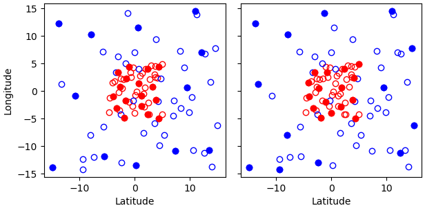
Fig. 23 Results of running the Poisson-disk thinning filter on sample data with the above parameters and two different random seeds. All observations have the same scan index. Observations with priorities 1 and 0 are marked with red and blue circles, respectively. Circles denoting retained observations are filled; those denoting rejected observations are empty. Note how blue (low-priority) observations are retained only in regions without red (high-priority) observations.

Example 2

With the following parameters, observations are thinned by the horizontal position, vertical position and time. The exclusion volumes are ellipsoidal. Shuffling is disabled.

- filter: Poisson Disk Thinning
  min_horizontal_spacing: 1000 # km
  min_vertical_spacing: 10000 # Pa
  min_time_spacing: PT1H
  exclusion_volume_shape: ellipsoid
  shuffle: false

Example 3

With the following parameters, observations are thinned by selecting the median observation within an exclusion volume.

- filter: Poisson Disk Thinning
  filter variables:
  - name: waterTemperature
  min_horizontal_spacing: 50
  shuffle: false
  select median: true

Duplicate Thinning Filter

The DuplicateThinning filter identifies duplicate observations within groups defined by one or more grouping variables and thins them based on time.

First the filter identifies groups of observations that fall into the same group bin based on the variable names parameter. For float variables, values are rounded to integer bins based on \(\text{bin} = \text{lround}\left(\frac{\text{value}}{\text{tolerance}}\right)\) using the corresponding tolerance parameter. This bin is then split into groups. For non-float variables, they are grouped by exact match, but the tolerance parameters need to be set, since there is a check to match the number of tolerance and variable names.

Second each group is sorted by dateTime and analysis_time window is applied: observations whose dateTime lies within analysis_time_tolerance are kept, while the others are flagged as thinned. The default analysis_time is the start of assimilation window and default analysis_time_tolerance of PT0H disables windowing.

Third, the filter applies temporal thinning within each group using min_spacing. The default value of min_spacing is PT6H, which means that if two observations in the same group are taken within 6 hours of each other, only one of them will be retained. When multiple observations in the same group fall within min_spacing of each other, only one observation is retained. The retained observation is selected based on proximity to analysis_time. If two observations are equidistant from analysis_time, equidistant_time_selection controls which one is retained. The default value, after, retains the observation after analysis_time; before retains the observation before analysis_time.

The observtions that are not grouped with any observations are temporally thinned based on their proximity to analysis_time.

Finally all flagged observations have their QCflags set to QCflags::thinned. The flagged observations are not removed from the observation space, unless specifed by the action parameter. If the action parameter is set to “reduce obs space”, the observations flagged as thinned are removed.

As with other QC filters, see Where Statement to limit which observations are considered by the filter.

Example:

- filter: DuplicateThinning
  simulated variables: [airTemperature]
  analysis_time: 2024-05-06T00:00:00Z
  analysis_time_tolerance: PT0S
  min_spacing: PT90M
  equidistant_time_selection: "after"
  variable names:
  - MetaData/stationIdentification
  - MetaData/longitude
  - MetaData/latitude
  - MetaData/height
  tolerance:
  - 1
  - 0.0001
  - 0.0001
  - 0.0001
  action:
    name: reduce obs space

Stuck Check Filter

This filter works record-by-record. Record grouping is therefore fundamental to its behavior. Records are usually defined with obs space.obsdatain.obsgrouping. See here for an example. If no obsgrouping is set, all valid observations are treated as one record.

Within each record and for each filter variables independently, the filter searches for streaks of consecutive identical values, excluding any missing values.

Consider a timeseries of \(N\) observations. A set of \(k \leq N\) identical observations in a row (skipping any missing values) is considered a streak which is which is used in one of the following ways:

• Mode A (count + time): uses a fixed number stuck tolerance \(T_{ns}\) and a time stuck tolerance to determine if a streak is “stuck”.

• Mode B (percentage): derives a number stuck tolerance \(T_{ns}\) from a percentage of observations in the record to determine if a streak is “stuck”. Does not use a time stuck tolerance.

Mode A: count + time mode

Required parameters:

• number stuck tolerance: a non-negative integer tolerance \(T_{ns}\) applied to streak intervals. A streak needs at least \(T_{ns} + 1\) identical observations in a row to be classified as “stuck”. Exactly one of number stuck tolerance and number stuck tolerance variable must be set in this mode.

• number stuck tolerance variable: a variable (for example in MetaData) containing integer tolerances \(T_{ns}\), allowing different tolerances for each record. For each record, all non-missing values of this variable must be identical and non-negative; records with all-missing values are skipped. Exactly one of number stuck tolerance and number stuck tolerance variable must be set in this mode.

• time stuck tolerance: the maximum allowed duration a streak satisfying \(k \ge T_{ns} + 1\) can be before being considered “stuck”. This parameter must be entered in ISO 8601 duration format. A streak is rejected as “stuck” only if its duration is strictly greater than time stuck tolerance. If the streak spans the full record, time stuck tolerance is ignored and the streak is rejected as “stuck”.

Mode B: percentage mode

Required parameter:

• percentage stuck tolerance: tolerance given as a percentage (from 0 to 100). This is converted to a per-record interval number stuck tolerance \(T_{ns}\).

  If percentage stuck tolerance based on intervals is false (default):

  \[T_{ns} = \mathrm{round}(p/100 \cdot N)\]

  If percentage stuck tolerance based on intervals is true:

  \[T_{ns} = \mathrm{round}(p/100 \cdot (N-1))\]

  where \(p\) is percentage stuck tolerance and \(N\) is the number of observations in the record.

Optional parameters in this mode:

• minimum allowed stuck: used with percentage stuck tolerance. If computed \(T_{ns}\) is strictly less than minimum allowed stuck, that record is skipped (no stuck rejections from that record). Default: 1 (two identical observations in a row).

• percentage stuck tolerance based on intervals: used with percentage stuck tolerance. If set to false (default), the percentage is applied to the number of observations in the record. If set to true, the percentage is applied to the number of intervals between observations in the record.

Validation rules

If percentage stuck tolerance is defined, then number stuck tolerance, number stuck tolerance variable, and time stuck tolerance must NOT be defined.

If percentage stuck tolerance is not defined, then time stuck tolerance must be defined and exactly one of number stuck tolerance or number stuck tolerance variable must be defined.

Examples 1, 2 and 3 illustrate Mode A. Examples 4, 5 and 6 illustrate Mode B.

Example 1

With the following parameters, a “streak” of observations is defined as sequential observations with identical air temperature measured values. All observations in the streak will be flagged if the streak (a) has at least 3 identical observations in a row and (b) lasts longer than 2 hours or consists of the full set of observations from the group (typically a station).

- filter: Stuck Check
  filter variables: [airTemperature]
  number stuck tolerance: 2
  time stuck tolerance: PT2H

Here \(T_{ns} = 2\), so the streak must satisfy \(k \ge T_{ns} + 1 = 3\).

Example 2

With the following parameters, 2 types of streaks will be identified independently and the observations will be flagged accordingly if either of the following observed values are classified as “stuck”: air temperature and air pressure.

- filter: Stuck Check
  filter variables: [airTemperature, pressure]
  number stuck tolerance: 2
  time stuck tolerance: PT2H

Again \(T_{ns} = 2\), so each variable needs at least 3 identical observations in a row.

Say we have 5 observations each taken an hour apart. Let the air temperature values be 274, 274, 274, 275, 275 and the air pressure values be 4, 4, 5, 5, 5. Each variable has 3 identical observations in a row (\(k = 3\)), meeting the length criterion (\(k \ge T_{ns} + 1\) with \(T_{ns}=2\)), but the duration is exactly 2 hours and therefore not strictly greater than PT2H. In this case, no observations are rejected.

Were the time stuck tolerance set to PT1H, the first three observations of air temperature and the last three observations of air pressure, which cover a duration of 2 hours, would be identified as “stuck” and be rejected.

Example 3

With the following parameters, the filter uses a per-record integer tolerance variable. For each record, all non-missing values of MetaData/numberStuckToleranceVariable must be equal.

- filter: Stuck Check
  filter variables: [windNorthward]
  number stuck tolerance variable: MetaData/numberStuckToleranceVariable
  time stuck tolerance: PT2M

Example values for MetaData/numberStuckToleranceVariable across two records:

• Record A (5 observations): [2, 2, 2, 2, 2] means \(T_{ns} = 2\), so at least 3 identical values in a row are needed.

• Record B (4 observations): [1, 1, 1, 1] means \(T_{ns} = 1\), so at least 2 identical values in a row are needed.

Example 4

In this example the number stuck tolerance \(T_{ns}\) is derived from a percentage of the number of observations in the record:

- filter: Stuck Check
  filter variables: [airTemperature]
  percentage stuck tolerance: 50

Using defaults (minimum allowed stuck: 1, percentage stuck tolerance based on intervals: false):

• If record A has \(N = 5\) observations, then \(T_{ns} = \mathrm{round}(0.5 \cdot 5) = 3\). A streak will be considered “stuck” if it has \(k \ge 4\) identical observations.

• Record B has \(N = 4\), so \(T_{ns} = \mathrm{round}(0.5 \cdot 4) = 2\). A streak will be considered “stuck” if it has \(k \ge 3\) identical observations.

If record A is 274, 274, 274, 274, 275 and record B is 274, 274, 275, 275, the first four observations in record A are rejected as “stuck”.

Example 5

With percentage-based tolerance, minimum allowed stuck can change the result by skipping records whose computed number stuck tolerance \(T_{ns}\) is too small.

- filter: Stuck Check
  filter variables: [airTemperature]
  percentage stuck tolerance: 25
  minimum allowed stuck: 2

Using percentage stuck tolerance based on intervals: false (default):

• Record A with \(N = 5\): \(T_{ns} = \mathrm{round}(0.25 \cdot 5) = 1\)

• Record B with \(N = 4\): \(T_{ns} = \mathrm{round}(0.25 \cdot 4) = 1\)

Because \(T_{ns} = 1 <\) minimum allowed stuck: 2, both records are skipped. If minimum allowed stuck were left at its default (1), these records would be checked.

Example 6

The percentage stuck tolerance based on intervals option changes the base of the calculation.

- filter: Stuck Check
  filter variables: [airTemperature]
  percentage stuck tolerance: 25
  percentage stuck tolerance based on intervals: true

For a record with \(N = 6\) observations:

• If percentage stuck tolerance based on intervals: false, \(T_{ns} = \mathrm{round}(0.25 \cdot 6) = 2\), so at least 3 identical observations are needed.

• If percentage stuck tolerance based on intervals: true, \(T_{ns} = \mathrm{round}(0.25 \cdot 5) = 1\), so at least 2 identical observations are needed.

Difference Check Filter

This filter will compare the difference between a reference variable and a second variable and assign a QC flag if the difference is outside of a prescribed range.

For example:

- filter: Difference Check
  reference: ObsValue/brightnessTemperature_8
  value: ObsValue/brightnessTemperature_9
  minvalue: 0

The above YAML is checking the difference between ObsValue/brightnessTemperature_9 and ObsValue/brightnessTemperature_8 and rejecting negative values.

In pseudo-code form: if (ObsValue/brightnessTemperature_9 - ObsValue/brightnessTemperature_8 < minvalue) reject_obs()

The options for YAML include:

• minvalue: the minimum value the difference value - reference can be. Set this to 0, for example, and all negative differences will be rejected.

• maxvalue: the maximum value the difference value - reference can be. Set this to 0, for example, and all positive differences will be rejected.

• threshold: the absolute value the difference value - reference can be (sign independent). Set this to 10, for example, and all differences outside of the range from -10 to 10 will be rejected.

Note that threshold supersedes minvalue and maxvalue in the filter.

The YAML may also include list of channels whose differences are to be checked. For example:

- filter: Difference Check
  reference:
    name: Hofx/brightnessTemperature
    channels: 1,3,5,7
  value:
     name: ObsValue/brightnessTemperature
     channels: 1,3,5,7
  minvalue: -2.5

In this case, the filter will check the difference between ObsValue/brightnessTemperature and Hofx/brightnessTemperature of channels 1, 3, 5, and 7, and flag the varaibles at all locations if the difference is less than the minvalue of -2.5.

If the difference happens be exactly equal to minvalue or maxvalue, the default behavior for this filter is for it to pass QC. (i.e. The passing range of values is inclusive of the endpoints.) This behavior can be changed by setting the min_exclusive and/or max_exclusive parameters to true, in which case differences equal to the specified limits will be rejected. For example, the following filter rejects all differences that are less than or equal to 0:

- filter: Difference Check
  reference: ObsValue/brightnessTemperature_8
  value: ObsValue/brightnessTemperature_9
  minvalue: 0
  min_exclusive: true

Derivative Check Filter

This filter will compute a local derivative over each observation record and assign a QC flag if the derivative is outside of a prescribed range.

By default, this filter will compute the local derivative at each point in a record.

• For the first location (1) in a record: dy/dx = (y(2)-y(1))/(x(2)-x(1))

• For the last location (n) in a record: dy/dx = (y(n)-y(n-1))/(x(n)-x(n-1))

• For all other locations (i): dy/dx = (y(i+1)-y(i-1))/(x(i+1)-x(i-1))

Alternatively if one wishes to use a specific range/slope for the entire observation record, i1 and i2 can be defined in the YAML. For this case, For all locations in the record: dy/dx = (y(i2)-y(i1))/(x(i2)-x(i1))

Note that this filter really only works/makes sense for observations that have been sorted by the independent variable and grouped by some other field.

An example:

- filter: Derivative Check
  independent: datetime
  dependent: pressure
  minvalue: -50
  maxvalue: 0
  passedBenchmark:  238      # number of passed obs

The above YAML is checking the derivative of pressure with respect to datetime for a radiosonde profile and rejecting observations where the derivative is positive or less than -50 Pa/sec.

The options for YAML include:

• independent: the name of the independent variable (dx)

• dependent: the name of the dependent variable (dy)

• minvalue: the minimum value the derivative can be without the observations being rejected

• maxvalue: the maximum value the derivative can be without the observations being rejected

• i1: the index of the first observation location in the record to use

• i2: the index of the last observation location in the record to use

A special case exists for when the independent variable is ‘distance’, meaning the dx is computed from the difference of latitude/longitude pairs converted to distance.

Additionally, when the independent variable is ‘datetime’ and the dependent variable is set to ‘distance’, the derivative filter becomes a speed filter, removing moving observations when the horizontal speed is outside of some range.

Spike and Step Check Filter

This filter goes through each record and flags observations where the value of the dependent variable (as specified by the user) is classified as a spike or step relative to adjacent points along the (user-specified) independent variable, e.g. profiles of ocean temperature against depth. (Only tested for data grouped into records - set grouping with the obs space.obsdatain.obsgrouping.group_variable YAML option. An example of its use can be found in the Profile consistency checks section.)

For a less profile-focused alternative, see Step Check.

A spike is a point whose dependent variable value differs from the adjacent points on either side of it by more than a given tolerance. A step is when two adjacent points’ dependent variable values differ from each other by more than the tolerance. The tolerance can vary along the independent variable (more below). Points only count as spikes or steps if they are isolated, and not part of a trend spanning multiple points. A spike results in the point in question being flagged; a step results in both points on either side of the step being flagged.

Required parameters:

• independent: the independent (\(x\)) variable, e.g. depth in ocean profiles. (Must be float type.)

• dependent: the dependent (\(y\)) variable, e.g. temperature or salinity in ocean profiles. (Must be float type.) NB: only one of each must be given.

• tolerance.nominal value: the tolerance value where \(x = 0\). The tolerance is the value against which adjacent differences \(dy\) in the dependent variable are compared, to determine whether points are spikes or steps.

Optional parameters:

• count spikes: If false, do not count spikes. Default: true.

• count steps: If false, do not count steps. Default: true.

• tolerance.threshold: For checking conditions for a large spike or large consistent gradient. The smaller tolerance.threshold is, the more symmetrical a spike must be to be considered a spike, and the more tightly the point must be aligned with the points on either side to be considered a consistent gradient (in which case the point would not be considered a spike). Default: \(0.5\).

• tolerance.gradient: \(dy/dx\) tolerance. If a point doesn’t meet the conditions for a large spike, it may yet count as a small spike if its gradient on either side exceeds the gradient tolerance (plus other conditions). Default: numeric maximum, i.e. nothing can exceed the gradient tolerance - small spikes are not counted if this option is left out.

• tolerance.gradient x resolution: precision of \(dx\) when calculating \(dy/dx\). Default: epsilon, i.e. the smallest possible to avoid a divide by \(0\) error.

• tolerance.factors and tolerance.x boundaries: vector floats of respectively the multiplier factors and \(x\)-points which when joined by straight line segments, determine the tolerance against \(x\): tolerance equals nominal tolerance multiplied by this line segment function thus defined. Either both factors and x boundaries must be given and of the same size, or neither given. x boundaries must be given in order of increasing \(x\) (and factors must match up with them). Default: nominal tolerance applies across whole \(x\) domain if neither are given.

• boundary layer.x range: a 2-element vector [min, max] defining the \(x\)-domain, min\(\le x <\)max, such that within it, the tolerance is modified (see step tolerance range below). Default: {0, 0}.

• boundary layer.step tolerance range: if \(x\) is within the boundary layer defined by boundary layer.x range, then if the adjacent difference \(dy\) is within the range defined by this 2-element vector step tolerance range, it cannot count as a step. Default: {0, 0}.

• boundary layer.maximum x interval: a 2-element vector [within, outside] such that if the spacing \(dx\) between two points is greater than the first element (when \(x\) within the boundary layer.x range) or the second (when \(x\) outside the boundary layer.x range), then ignore the corresponding \(dy\); do not check if it is a spike or step. Default: {numeric max, numeric max}, i.e. check every observation.

A call to Spike and Step Check MUST be preceded by creating Diagnostic Flags for the dependent variables in question, and the flags MUST be named “spike” and “step”:

- filter: Create Diagnostic Flags
  filter variables:
    - name: waterTemperature
    - name: salinity
  flags:
  - name: spike
    initial value: false
  - name: step
    initial value: false

This is because the Spike and Step Check sets these flags separately within the code itself. The flags thus set can then be used in the YAML, e.g. to count how many spikes and steps are in each record, and reject entire records whose sum of spikes and steps exceeds a given threshold. An example of this can be found in qc_spike_and_step_check.yaml

An example of applying the Spike and Step Check filter:

- filter: Spike and Step Check
  filter variables:
    - name: ObsValue/waterTemperature
  dependent: ObsValue/waterTemperature  # dy/
  independent: MetaData/depthBelowWaterSurface      # dx
  count spikes: true
  count steps: true
  tolerance:
    nominal value: 10  # K, in the case of temperature (not real value)
    gradient: 0.1      # K/m - if dy/dx greater, could be a spike
    gradient x resolution: 10       # m - can't know dx to better precision
    factors: [1.0, 1.0, 0.5, 0.5, 0.1]        # multiply tolerance, for ranges bounded by...
    x boundaries: [0, 200, 300, 600, 600] # ...these values of x (depth in m)
  boundary layer:
    x range: [0.0, 300.0]               # when bounded by these x values (depth in m)...
    step tolerance range: [-1.0, -2.0]  # ...relax tolerance for steps in boundary layer...
    maximum x interval: [50.0, 100.0]   # ...and ignore level if dx greater than this
  action:
    name: reject

In this case, both spikes and steps are counted for waterTemperature profiles, and rejected for waterTemperature only, since that is the only filter variable listed. If other filter variables were listed, they would all be rejected at locations where spikes and steps in waterTemperature (the dependent variable) are found. If looking for spikes and steps in other variables, the Spike and Step Check needs to be called again on each of them as the dependent variable separately.

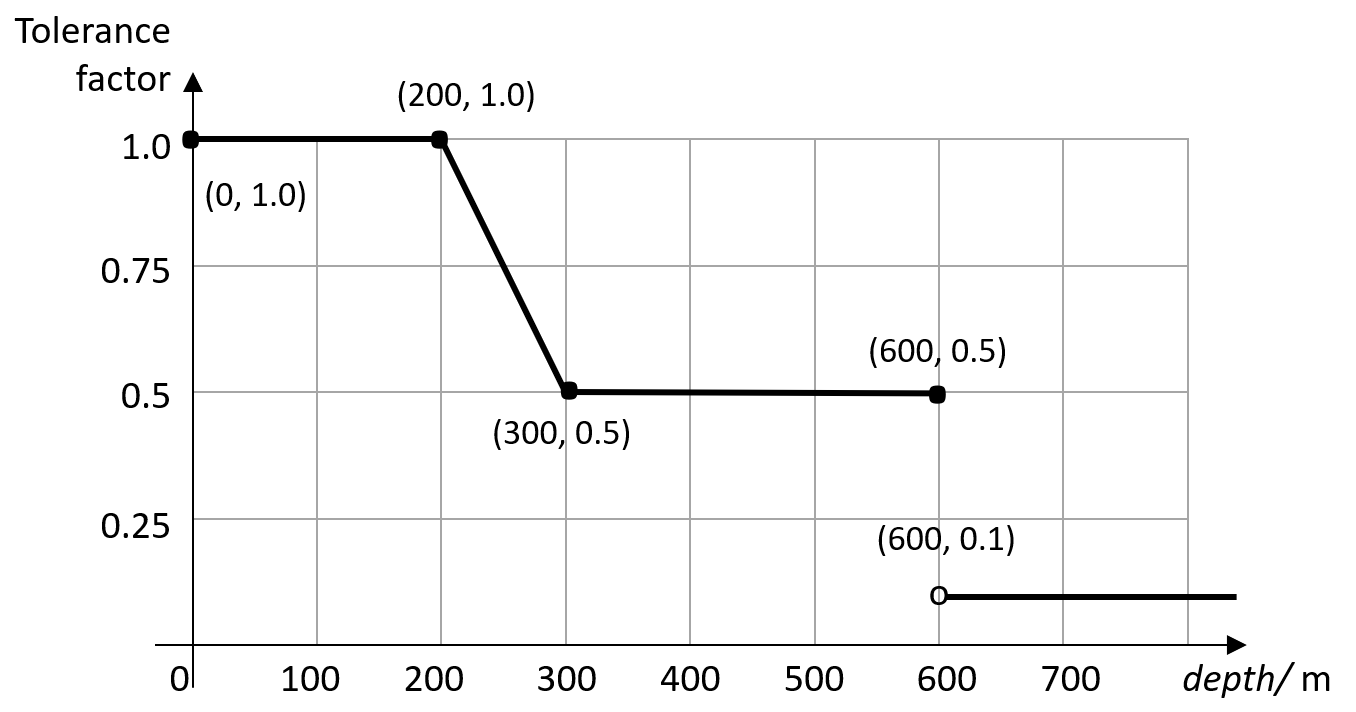
Fig. 24 The tolerance function specified by tolerance.factors and tolerance.x boundaries: straight line segments joining \((0, 1.0)\), \((200, 1.0)\), \((300, 0.5)\), \((600, 0.5)\), \((600, 0.1)\), and constant at \(0.1\) subsequently.

The tolerance value as a function of \(x\), is the nominal value (\(10\) K) multiplied by the tolerance factor function. In this example, the filter is more sensitive to spikes and steps the deeper you go. Note that tolerance function is constant at the last value in factors when \(x\) exceeds the last value in x boundaries. For jumps in tolerance such as at \(x = 600\) m, the value on the left hand side (smaller \(x\)) is used.

The temperature gradient (in K/m) is computed for each profile, and any point that does not count as a large spike but whose gradient on either side exceeds the gradient tolerance \(0.1\) K/m (amongst other conditions), is counted as a small spike. (The flagging does not distinguish between large and small spikes, they are all spikes.) For any points separated by less than \(10\) m (gradient x resolution), the gradient is computed as the dependent variable adjacent difference \(dy\) divided by \(10\) m, preserving the sign of \(dx\).

The boundary layer is defined by boundary layer.x range to be 0\(\le x <\)300 m. When \(x\) is within the boundary layer, a step is unflagged if \(dy\) is within the step tolerance range multiplied by the tolerance function - as shown in the figure below:

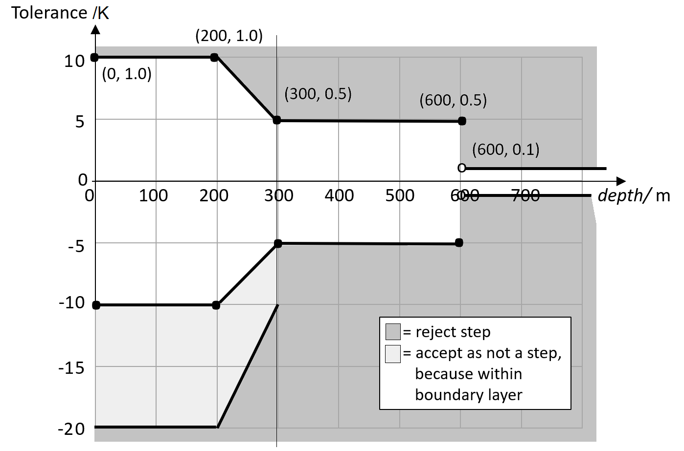
Fig. 25 Adjacent points with \(dy\) exceeding the tolerance (positive or negative) are flagged as steps; but if \(x\) is within the boundary layer, the tolerance to steps is relaxed by the factors given in step tolerance range.

If two adjacent points have \(y\) value differing by more than the tolerance at their level \(x\), and if neither is a spike nor part of a large consistent gradient, they are flagged as a step (i.e. if \(dy\) is in the dark grey region). However, the condition is more lenient within the boundary layer, 0\(\le x <\)300 m: the points are accepted as not a step if their \(dy\) falls within the light grey region, which is \(-1\) to \(-2\) times the tolerance (boundary layer.step tolerance range: [-1.0, -2.0]).

Additionally, if the spacing \(dx\) between adjacent points is \(> 50\) m while \(x\) within the boundary layer, then the corresponding \(dy\) is skipped when checking for spikes and steps. That is, points spaced too far apart cannot be confidently flagged as spikes or steps. Outside of the boundary layer, the condition is applied when \(dx > 100\) m, as boundary layer.maximum x interval: [50.0, 100.0].

The reason for the boundary layer options section is to accomodate a thermocline or halocline in the ocean, where a large negative gradient is expected and is not cause to flag a step, unless very large indeed, or large and positive. There is no impact on spike flagging. If the section is left out, the rest of the code applies, there is no relaxation of tolerance conditions anywhere.

Note that this filter does not currently support use of “where” clauses.

Track Check Filter

This filter checks tracks of mobile weather stations, rejecting observations inconsistent with the rest of the track.

Each track is checked separately. The algorithm performs a series of sweeps over the observations from each track. For each observation, multiple estimates of the instantaneous speed and (optionally) ascent/descent rate are obtained by comparing the reported position with the positions reported during a number a nearby (earlier and later) observations that haven’t been rejected in previous sweeps. An observation is rejected if a certain fraction of these estimates lie outside the valid range. Sweeps continue until one of them fails to reject any observations, i.e. the set of retained observations is self-consistent.

Note that this filter was originally written with aircraft observations in mind. However, it can potentially be useful also for other observation types.

The following YAML parameters are supported:

• temporal_resolution: Assumed temporal resolution of the observations, i.e. absolute accuracy of the reported observation times. Default: PT1M.

• spatial_resolution: Assumed spatial resolution of the observations (in km), i.e. absolute accuracy of the reported positions.

  Instantaneous speeds are estimated conservatively with the formula

  speed_estimate = (reported_distance - spatial_resolution) / (reported_time + temporal_resolution).

  The default spatial resolution is 1 km.

• num_distinct_buddies_per_direction, distinct_buddy_resolution_multiplier: Control the size of the set of observations against which each observation is compared.

  Let O_i (i = 1, …, N) be the observations from a particular track ordered chronologically. Each observation O_i is compared against m observations immediately preceding it and n observations immediately following it. The number m is chosen so that {O_{i-m}, …, O_{i-1}} is the shortest sequence of observations preceding O_i that contains num_distinct_buddies_per_direction observations distinct from O_i that have not yet been rejected. Two observations taken at times t and t’ and locations x and x’ are deemed to be distinct if the following conditions are met:

  • |t’ - t| > distinct_buddy_resolution_multiplier * temporal_resolution

  • |x’ - x| > distinct_buddy_resolution_multiplier * spatial_resolution

  Similarly, the number n is chosen so that {O_{i+1}, …, O_{i+n)} is the shortest sequence of observations following O_i that contains num_distinct_buddies_per_direction observations distinct from O_i that have not yet been rejected.

  Both parameters default to 3.

• max_climb_rate: Maximum allowed rate of ascent and descent (in Pa/s). If not specified, climb rate checks are disabled.

• max_speed_interpolation_points: Encoding of the function mapping air pressure (in Pa) to the maximum speed (in m/s) considered to be realistic.

  The function is taken to be a linear interpolation of a series of (pressure, speed) points. The pressures and speeds at these points should be specified as keys and values of a JSON-style map. Owing to a bug in the eckit YAML parser, the keys must be enclosed in quotes. For example,

  max_speed_interpolation_points: { "0": 900, "100000": 100 }
  

  encodes a linear function equal to 900 m/s at 0 Pa and 100 m/s at 100000 Pa.

• rejection_threshold: Maximum fraction of climb rate or speed estimates obtained by comparison with other observations that are allowed to fall outside the allowed ranges before an observation is rejected. Default: 0.5.

• station_id_variable: Variable storing string- or integer-valued station IDs. Observations taken by each station are checked separately.

  If not set and observations were grouped into records when the observation space was constructed, each record is assumed to consist of observations taken by a separate station. If not set and observations were not grouped into records, all observations are assumed to have been taken by a single station.

  Note: the variable used to group observations into records can be set with the obs space.obsdatain.obsgrouping.group_variable YAML option.

Example:

- filter: Track Check
  temporal_resolution: PT30S
  spatial_resolution: 20 # km
  num_distinct_buddies_per_direction: 3
  distinct_buddy_resolution_multiplier: 3
  max_climb_rate: 200 # Pa/s
  max_speed_interpolation_points: {"0": 1000, "20000": 400, "110000": 200} # Pa: m/s
  rejection_threshold: 0.5
  station_id_variable: MetaData/stationIdentification

Ship Track Check Filter

This filter checks tracks of mobile weather stations, rejecting observations inconsistent with the rest of the track. It differs from Track Check Filter in that it only considers inconsistencies in the lat-lon and time dimensions of each observation.

Each track is checked separately. The algorithm starts by performing the following calculations between consecutive observations:

1. Distances between each observation

2. The speed between each observation

3. Angles of the track formed by each triplet of consecutive observations

Various track statistics will be calculated:

1. The number of track segments (tracks between two consecutive observations) with less than an hour between the two observations.

2. The number of track segments which exceed a user-defined maximum speed.

3. The average speed of all track segments which do not fall into categories (1) and (2).

4. The number of track angles which are greater than or equal to 90 degrees.

If (1), (2), and (4) exceed a percentage of the total observations and the user-defined early break check setting is enabled, then the track is skipped over, with all observations left unflagged.

If the filter proceeds, observations are flagged iteratively by removing one of the two observations forming the fastest segment, until either (a) the segment with the fastest speed is less than a user-defined max speed (m/s) and the angles formed by this segment with its adjacent segments are both less than 90 degrees or (b) the segment with the fastest speed is less than 80 percent of max speed (m/s).

Numerous criteria are applied to choose which of the two observations forming the fastest track segment should be removed, and track statistic (3) is heavily used in this assessment. If the percentage of observations rejected rises greater than a user-defined rejection threshold fraction, the full track is rejected.

The following YAML parameters are supported:

• temporal resolution: Assumed temporal resolution of the observations (i.e. absolute accuracy of the reported observation times). Used as the time interval for the speed calculations if it is greater than the reported time between two consecutive observations; otherwise the reported time is used. Required parameter.

• spatial resolution (km): Assumed spatial resolution of the observations (in km), i.e. absolute accuracy of the reported positions. Required parameter.

• max speed (m/s): The maximum speed (in m/s) between any two observations, above which requires the rejection of one of the comprising observations. Required parameter.

• rejection threshold: The maximum fraction of track observations to be rejected, above which causes the full track to be rejected. Required parameter.

• early break check: A boolean setting that determines if a track should be skipped (unfiltered) if its count of track statistics (1), (2), and (4) are too large a percentage of the total number of observations. Required parameter.

• input category: The type of input source. If a static source such as BUOY, track statistic (1) will not be considered in deciding if a track should be skipped. Default: SHPSYN. The supported sources are: LNDSYN, SHPSYN, BUOY, MOBSYN, OPENROAD, TEMP, BATHY, TESAC, BUOYPROF, LNDSYB, and SHPSYB.

• records_are_single_obs: If true, then treat each record as a single location within the track - accept or reject entire records according to the above criteria. Default: false. If option set to true while observations are not grouped into records, an error will be thrown. Set grouping with the obs space.obsdatain.obsgrouping.group_variable YAML option. An example of its use can be found in the Profile consistency checks section.

• station_id_variable: The variable that defines the tracks - note that this may be different from the obs grouping variable(s) that define records (there may be multiple records per track). If not given and if records_are_single_obs: true OR if not given while not grouped into records at all, then all the observations (records or individual) are treated as belonging to a single continuous track. However, if not given while grouped into records but records_are_single_obs: false, then each record is treated as a separate track.

Example:

- filter: Ship Track Check
  temporal resolution: PT30S
  spatial resolution (km): .1
  max speed (m/s): 3.0
  rejection threshold: 0.5
  station_id_variable:
    name: MetaData/stationIdentification
  records_are_single_obs: true

Met Office Buddy Check Filter

This filter cross-checks observations taken at nearby locations against each other, updating their gross error probabilities (PGEs) and rejecting observations whose PGE exceeds a threshold specified in the filter parameters. For example, if an observation has a very different value than several other observations taken at nearby locations and times, it is likely to be grossly in error, so its PGE is increased. PGEs obtained in this way can be taken into account during variational data assimilation to reduce the weight attached to unreliable observations without necessarily rejecting them outright.

The YAML parameters supported by this filter are listed below.

• General parameters:

  • filter variables (a standard parameter supported by all filters): List of the variables to be checked. Surface data, single-level and multi-level variables. are supported. Variables can be either scalar or vector (with two Cartesian components, such as the eastward and northward wind components). In the latter case the two components need to be specified one after the other in the filter variables list, with the first component having the first_component_of_two option set to true. Example:

    filter variables:
    - name: airTemperature
    - name: windEastward
      options:
        first_component_of_two: true
    - name: windNorthward
    

  • rejection_threshold: Observations will be rejected if the gross error probability lies at or above this threshold. Default: 0.5.

  • traced_boxes: A list of quadrangles bounded by two meridians and two parallels. Tracing information (potentially useful for debugging) will be output for observations lying within any of these quadrangles. Example:

    traced_boxes:
      - min_latitude: 30
        max_latitude: 45
        min_longitude: -180
        max_longitude: -150
      - min_latitude: -45
        max_latitude: -30
        min_longitude: -180
        max_longitude: -150
    

    Default: empty list.

• Buddy pair identification:

  • num_levels: Number of levels. Optional parameter.

    This would not be specified for surface fields. It should be set to 1 for single level fields and be set to >1 for multi-level fields (i.e. corresponding to the number of levels).

  • search_radius: Maximum distance between two observations that may be classified as buddies, in km. Default: 100 km.

  • station_id_variable: Variable storing string- or integer-valued station IDs.

    If not set and observations were grouped into records when the observation space was constructed, each record is assumed to consist of observations taken by a separate station. If not set and observations were not grouped into records, all observations are assumed to have been taken by a single station.

    Note: the variable used to group observations into records can be set with the obs space.obsdatain.obsgrouping.group_variable YAML option. An example of its use can be found in the Profile consistency checks section above.

  • override_obs_grouping: Override observation space grouping (default true).

    If the observation space has been divided into records according to at least one grouping variable then, by default, the multi-level buddy check will be performed. However, if the parameter num_levels is equal to 1, the division into records is disregarded if the parameter override_obs_grouping is set to true. In that case individual observations are treated separately in the buddy check. The value of override_obs_grouping only has an effect if num_levels has been set to 1. In all other cases it is ignored.

  • num_zonal_bands: Number of zonal bands to split the Earth’s surface into when building a search data structure.

    Note: Apart from the impact on the speed of buddy identification, both this parameter and sort_by_pressure affect the order in which observations are processed and thus the final estimates of gross error probabilities, since the probability updates made when checking individual observation pairs are not commutative.

    Default: 24.

  • sort_by_pressure: Whether to include pressure in the sorting criteria used when building a search data structure, in addition to longitude, latitude and time. See the note next to num_zonal_bands. Default: false.

  • max_total_num_buddies: Maximum total number of buddies of any observation.

    Note: In the context of this parameter, max_num_buddies_from_single_band and max_num_buddies_with_same_station_id, the number of buddies of any observation O is understood as the number of buddy pairs (O, O’) where O’ != O. This definition facilitates the buddy check implementation (and makes it compatible with the original version from the OPS system), but is an underestimate of the true number of buddies, since it doesn’t take into account pairs of the form (O’, O).

    Default: 15.

  • max_num_buddies_from_single_band: Maximum number of buddies of any observation belonging to a single zonal band. See the note next to max_total_num_buddies. Default: 10.

  • max_num_buddies_with_same_station_id: Maximum number of buddies of any observation sharing that observation’s station ID. See the note next to max_total_num_buddies. Default: 5.

  • use_legacy_buddy_collector: Set to true to identify pairs of buddy observations using an algorithm reproducing exactly the algorithm used in Met Office’s OPS system, but potentially skipping some valid buddy pairs. Default: false.

• Control of gross error probability updates:

  • horizontal_correlation_scale: Encoding of the function that maps the latitude (in degrees) to the horizontal correlation scale (in km).

    The function is taken to be a piecewise linear interpolation of a series of (latitude, scale) points. The latitudes and scales at these points should be specified as keys and values of a JSON-style map. Owing to a limitation in the eckit YAML parser (https://github.com/ecmwf/eckit/pull/21), the keys must be enclosed in quotes. For example,

    horizontal_correlation_scale: { "-90": 200, "90": 100 }
    

    encodes a function varying linearly from 200 km at the south pole to 100 km at the north pole.

    Default: { "-90": 100, "90": 100 }, i.e. a constant function equal to 100 km everywhere.

  • horizontal_correlation_scale_2 (optional): In the same format as horizontal_correlation_scale, define a second latitude-dependent length scale to use in the calculation of the PGE adjustment. E.g. the oceans use mesoscale and synoptic length scales. N.B.: for this option to be used, both anisotropy, anisotropy_2 and background_error_group_2 must be specified (see below).

  • anisotropy: Latitude-dependent anisotropy factor, specified in the same format as horizontal_correlation_scale. Must be given if using 2-scale Buddy Check. A factor of 1 means isotropic; >1 means a buddy pair of observations a given distance apart would cause a greater PGE increase if the line joining them is aligned closer to an E-W line than to N-S. If not specified, the filter reverts to 1-scale isotropic.

  • anisotropy_2: As for anisotropy, but to match the second length scale. Must be given if using 2-scale Buddy Check. If not specified, the filter reverts to 1-scale isotropic.

  • temporal_correlation_scale: Temporal correlation scale. Default: PT6H.

  • vertical_correlation_scale: Vertical correlation scale which relates to the ratio of pressures. Default: 6.

  • damping_factor_1 Parameter used to “damp” gross error probability updates using method 1 described in section 3.8 of the OPS Scientific Documentation Paper 2 to make the buddy check better-behaved in data-dense areas. See the reference above for the full description. Default: 1.0.

  • damping_factor_2 Parameter used to “damp” gross error probability updates using method 2 described in section 3.8 of the OPS Scientific Documentation Paper 2 to make the buddy check better-behaved in data-dense areas. See the reference above for the full description. Default: 1.0.

  • background_error_group: Group name of the background error variable. Default: ObsDiag.

  • background_error_suffix: Suffix of the background error variable. Default: _background_error, i.e. if neither the group nor suffix are specified, the background error is assumed to be ObsDiag/<var>_background_error for the corresponding filter variable <var>.

  • background_error_group_2: As for background_error_group, but for the second length scale. If not specified, the filter reverts to 1-scale isotropic.

  • background_error_suffix_2: As for background_error_suffix, but for the second length scale. Default: "", e.g. if not specified but background_error_group_2: MesoscaleError, then the second background error is assumed to be MesoscaleError/<var> for the filter variable <var>.

Example:

- filter: Met Office Buddy Check:
  filter variables:
  - name: windEastward
    options:
      first_component_of_two: true
  - name: windNorthward
  - name: airTemperature
  rejection_threshold: 0.5
  traced_boxes: # trace all observations
  - min_latitude: -90
    max_latitude:  90
    min_longitude: -180
    max_longitude:  180
  search_radius: 100 # km
  station_id_variable:
    name: MetaData/stationIdentification
  num_zonal_bands: 24
  sort_by_pressure: false
  max_total_num_buddies: 15
  max_num_buddies_from_single_band: 10
  max_num_buddies_with_same_station_id: 5
  use_legacy_buddy_collector: false
  horizontal_correlation_scale: { "-90": 100, "90": 100 }
  temporal_correlation_scale: PT6H
  damping_factor_1: 1.0
  damping_factor_2: 1.0

Implementation Notes

The implementation of this filter consists of four steps: sorting, buddy pair identification, PGE update and observation flagging. Observations are grouped into zonal bands and sorted by (a) band index, (b) longitude, (c) latitude, in descending order, (d) pressure (if the sort_by_pressure option is on), and (e) datetime. Observations are then iterated over, and for each observation a number of nearby observations (lying no further than search_radius) are identified as its buddies. The size and “diversity” of the list of buddy pairs can be controlled with the max_total_num_buddies, max_num_buddies_from_single_band and max_num_buddies_with_same_station_id options. Subsequently, the PGEs of the observations forming each buddy pair are updated. Typically, the PGEs are decreased if the signs of the innovations agree and increased if they disagree. The magnitude of this change depends on the background error correlation between the two observation locations, the error estimates of the observations and background values, and the prior PGEs of the observations: the PGE change is the larger, the stronger the correlation between the background errors and the narrower the error margins. Once all buddy pairs have been processed, observations whose PGEs exceed the specified rejection_threshold are flagged.

In calculation of the background error correlation, for both surface and multi-level fields, a vertical correlation of 1 is assumed. For single-level data, the estimate of the background error correlation depends upon the ratio of pressures between each pair of observations.

History Check Filter

This filter runs the Ship Track Check Filter and/or the Stuck Check Filter (depending on the observation type) on an auxiliary obs space. The auxiliary obs space should be a superset of the original obs space, with an earlier start time than the assimilation window and either the same, or optionally a later, end time. The equivalent observations to those which were flagged in the auxiliary obs space are then flagged in the original obs space. This filter is motivated by the fact that the Ship Track Check and Stuck Check filters both rely on viewing observations within the context of their surrounding observations. Thus, this filter makes the underlying filters more reliable for observations close to the temporal boundaries of the assimilation window. The filters are run independently: any observations within the assimilation window flagged by either of the sub-filters will be flagged by this filter.

The following YAML parameters are supported:

• input category: Surface observation subtype which determines if the ship track check and/or the stuck check filters should be run. Supported options are LNDSYN, SHPSYN, BUOY, MOBSYN, OPENROAD, TEMP, BATHY, TESAC, BUOYPROF, LNDSYB, and SHPSYB. Required parameter.

• time before start of window: The duration of time before the start of the assimilation window to collect for the history check. This required parameter must be entered in ISO 8601 duration format.

• time after end of window: The duration of time after the end of the assimilation window to collect for the history check. This optional parameter must be entered in ISO 8601 duration format.

• ship track check parameters: The options for running the ship track check filter, should the subtype not be LNDSYN or LNDSYB. These must be filled in for the ship track check filter to run. The particular sub-parameters to fill in are temporal resolution, spatial resolution (km), max speed (m/s), rejection threshold, and early break check. Note that records_are_single_obs cannot be used in the History Check and will throw an error. Please refer to the Ship Track Check filter documentation for additional details on how each of these sub-parameters works. Optional parameter.

• stuck check parameters: The options for running the stuck check filter, should the subtype not be TEMP, BATHY, TESAC, or BUOYPROF. These must be filled in for the stuck check filter to run. The particular sub-parameters to fill in are number stuck tolerance and time stuck tolerance. Please refer to the Stuck Check Filter documentation for additional details on how each of these sub-parameters works. Optional parameter.

• obs space: The options used to create the auxiliary obs space that is determined by the observation subtype. A user needs to enter the following fields: name, simulated variables, and obsdatain. It additionally may be necessary to specify the distribution as InefficientDistribution. This prevents the observations from distributing to different processors between the original obs space and the auxiliary obs space, which could cause in-window observations flagged in the auxiliary obs space to be left unflagged in the original obs space. Required parameter.

• station_id_variable: Variable storing string- or integer-valued station IDs. Observations taken by each station are checked separately. Applies to assimilation observation space. Optional parameter.

  If not set and observations were grouped into records when the observation space was constructed, each record is assumed to consist of observations taken by a separate station. If not set and observations were not grouped into records, all observations are assumed to have been taken by a single station.

Example:

With the following parameters, the history check filter will be run on the obs space explicitly simulated, using the generated air temperature values for the stuck check and the lat-lon-dt values for the ship track check. time before start of window set as 3 hours will cause the filters to run from 3 hours before the start of the assimilation window (regardless of the time range present in the auxiliary obs space).

- filter: History Check
  input category: 'SHPSYN'
  time before start of window: PT3H
  filter variables: [airTemperature]
  stuck check parameters:
    number stuck tolerance: 2
    time stuck tolerance: PT2H
  ship track check parameters:
    temporal resolution: PT1S
    spatial resolution (km): 0.001
    max speed (m/s): 0.01
    rejection threshold: 0.5
    early break check: false
  station_id_variable:
    name: MetaData/stationIdentification
  obs space:
    name: Ship
    distribution: InefficientDistribution
    simulated variables: [airTemperature]
    generate:
      list:
        lats: [-37.1, -37.2, -37.3]
        lons: [82.5, 82.5, 82.5]
        datetimes: [ '2010-01-01T00:00Z', '2010-01-01T01:30Z', '2010-01-01T03:00Z']
      obs errors: [1.0]

Variable Assignment Filter

This “filter” (it is not a true filter; rather, a “processing step”) assigns specified values to specified variables at locations selected by the where statement, or at all locations if the where keyword is not present. The where operator parameter can be used to specify the logical operator used to combine conditions used in the where statement. The possible values are and (the default) and or. Note that it is possible to use the where operator option without the where statement. The option has no impact in that case.

The assigned values can be constants, existing ObsSpace variables or vectors generated by ObsFunctions. If the variables don’t exist yet, they are created; in this case locations not selected by the where statement are initialized with missing-value markers.

The values assigned to individual variables are specified in the assignments list in the YAML file. Each element of this list can contain the following options:

• name: Name of the variable to which new values should be assigned. The variable can be from any group except for ObsValue (use DerivedObsValue instead).

• channels: (Optional) Set of channels to which new values should be assigned.

• value: Value to be assigned to the specified variable. If this parameter is set to the string missing, the variable will be set to the relevant missing value at all locations that pass the where clause. The missing value to use is deduced from the type of the variable. Note it is therefore not possible to assign the string missing to a variable because it will be automatically converted to the missing string signifier. Exactly one of the value, source variable and function options must be present.

• source variable: Variable that should be copied into the destination variable (specified in the name option). Exactly one of the value, source variable and function options must be present.

• function: An ObsFunction that should be evaluated and assigned to the specified variable. Exactly one of the value, source variable and function options must be present.

• type: Type (int, float, string or datetime) of the variable to which new values should be assigned. This option only needs to be provided if the variable doesn’t exist yet. If this option is provided and the variable already exists, its type must match the value of this option, otherwise an exception is thrown.

• epoch: Date-time epoch used when converting values from a datetime source variable to a numeric destination variable (type int or float). The assigned numeric value is the number of seconds relative to this epoch. This option is required for datetime-to-numeric conversion and ignored otherwise.

When assigning from a source variable, a conversion exception is thrown if values cannot be converted to the destination type. For example, with a datetime-to-numeric conversion, this can happen if the chosen epoch makes the seconds offset too large for the destination numeric type.

It is possible to assign variables or ObsFunctions of type int to variables of type float and vice versa. No other type conversions are supported.

If the modified variable belongs to the DerivedObsValue group and is a observed variable, QC flags previously set to missing are reset to pass at locations where a valid observed value has been assigned. Conversely, QC flags previously set to pass are reset to missing at locations where the observed value has been set to missing.

Example 1

Create new variables GrossErrorProbability/airTemperature and GrossErrorProbability/relativeHumidity and set them to 0.1 at all locations.

- filter: Variable Assignment
  assignments:
  - name: GrossErrorProbability/airTemperature
    type: float  # type must be specified if the variable doesn't already exist
    value: 0.1
  - name: GrossErrorProbability/relativeHumidity
    type: float
    value: 0.1

Example 2

Set GrossErrorProbability/airTemperature to 0.05 at all locations in the tropics.

- filter: Variable Assignment
  where:
  - variable:
      name: MetaData/latitude
    minvalue: -30
    maxvalue:  30
  assignments:
  - name: GrossErrorProbability/airTemperature
    value: 0.05

Example 3

Set GrossErrorProbability/relativeHumidity to values computed by an ObsFunction (0.1 in the southern extratropics and 0.05 in the northern extratropics, with a linear transition in between).

- filter: Variable Assignment
  assignments:
  - name: GrossErrorProbability/relativeHumidity
    function:
      name: ObsFunction/ObsErrorModelRamp
      options:
        xvar:
          name: MetaData/latitude
        x0: [-30]
        x1: [30]
        err0: [0.1]
        err1: [0.05]

Example 4

Copy the variable MetaData/height to DerivedMetaData/geopotentialHeight.

- filter: Variable Assignment
  assignments:
  - name: DerivedMetaData/geopotentialHeight
    type: float  # type must be specified if the variable doesn't already exist
    source variable: MetaData/height

Example 5

Initialise the variable MetaData/pressure to the missing floating-point value at all locations.

- filter: Variable Assignment
  assignments:
  - name: MetaData/pressure
    type: float  # type must be specified if the variable doesn't already exist
    value: missing

Create Diagnostic Flags Filter

This “filter” (it is not a true filter; rather, a “processing step”) makes it possible to define new diagnostic flags and to reinitialize existing ones.

Diagnostic flags can be stored in two different ways:

• in Boolean ObsSpace variables. A diagnostic flag Flag associated with a observed variable var is stored in the variable DiagnosticFlags/Flag/var;

• in Integer ObsSpace variables (Integer serves as a bitmap). A diagnostic flag associated with an observed variable var is stored in the variable DiagnosticFlags/var.

The Boolean diagnostic flags to create or reinitialize are specified in the flags list in the YAML file. Each element of this list can contain the following keys:

• name (required): The flag name. Conventionally, flag names follow the CamelCase naming convention (like group names).

• initial value: Initial value for the flag (either true or false). If not specified, defaults to false.

• force reinitialization: Determines what happens if the flag already exists. By default, the flag is not reinitialized, i.e. its current value is preserved. Set force reinitialization to true to reset the flag to initial value.

The Integer (bitmap) diagnostic flags are created or reinitialized if bitmap diagnostic flags is set to true in the YAML file. force bitmap reinitialization option behaves similarly to force reinitialization for the bitmap diagnostics flags. Bitmap diagnostic flags are always set to zero on creation or reinitialization.

In addition, the filter recognizes the standard filter options filter variables and defer to post, but not where or action.

Setting and unsetting of diagnostic flags or bits of diagnostic flags (for the bitmap diagnostics) is normally performed using actions on a given filter; examples can be seen in Filter Actions.

Example 1

The following YAML snippet creates diagnostic flags Duplicate and ExtremeValue for all observed variables and initializes them to false unless they already exist, in which cause their current values are preserved.

- filter: Create Diagnostic Flags
  flags:
  - name: Duplicate
  - name: ExtremeValue

For instance, if the list of observed variables in the ObsSpace is [airTemperature, relativeHumidity], the filter will create the following Boolean variables: DiagnosticFlags/Duplicate/airTemperature, DiagnosticFlags/Duplicate/relativeHumidity, DiagnosticFlags/ExtremeValue/airTemperature and DiagnosticFlags/ExtremeValue/relativeHumidity.

Example 2

The following YAML snippet creates a diagnostic flag OriginallyMeasuredInMmHg for the observed variable stationPressure and initializes it to true, overwriting any current values if this flag already exists:

- filter: Create Diagnostic Flags
  filter variables: [stationPressure]
  flags:
  - name: OriginallyMeasuredInMmHg
    initial value: true
    force reinitialization: true

Example 3

The following YAML snippet creates bitmap diagnostic variable for the observed variable stationPressure.

- filter: Create Diagnostic Flags
  filter variables: [stationPressure]
  bitmap diagnostic flags: true

RTTOV 1D-Var Check (RTTOVOneDVar) Filter

This filter performs a 1-dimensional variational assimilation (1D-Var) that produces optimal retrievals of physical parameters that describe the atmosphere and surface on which there is information in the measurement. It takes as input a set of observations (brightness temperatures) and model background fields which are used to initialise the retrieval profile. A retrieval (or analysis) is performed using an iterative procedure that attempts to find the minimum of a cost function that represents the most likely profile vector given the error characteristics of the two data sources.

The elements contained in the retrieval profile depend on the sensitivity of the measuring instruments to atmospheric and surface properties and also what can be modelled with a relatively high degree of accuracy. Most retrieval profiles will consist of atmospheric temperature and humidity, and surface skin temperature, with other possible constituents being liquid and ice water or some other cloud parameter measure, and emissivity parameters.

The filter provides some retrieval parameters to the main assimilation which may be missing in the background or insufficiently accurate, such as surface skin temperature, and to filter out observations for which a retrieval could not be performed and thus may be difficult to assimilate in the full variational assimilation.

The filter is a port of the Met Office OPS 1D-Var and makes use of the Fortran RTTOV interface within JEDI. The code is written predominantly in Fortran. Files containing the observation error covariance (R) and the background error covariance (B) are expected as inputs.

This filter requires the following YAML parameters:

• BMatrix: path to the b-matrix file.

• RMatrix: path to the r-matrix file.

• nlevels: the number of levels used in the retrieval profile.

• retrieval variables from geovals: list of retrieval variables (e.g. temperature etc) which form the 1D-Var retrieval vector (x) and are provided by the model interface. These need to be in the b-matrix file.

• ModOptions: options needed for the observation operator (RTTOV only at the moment).

• filter variables: list of variables (brightnessTemperature) and channels which form the 1D-Var observation vector (y).

The following are optional YAML parameters with defaults listed where a variable has a default value:

• retrieval variables not from geovals: list of retrieval variables (e.g. pressureAtCloudTop etc) which form the 1D-Var retrieval vector (x) and are not provided by the model interface. These need to be in the ObsSpace and b-matrix file.

• ModName: forward model name (only RTTOV at the moment). Default: RTTOV.

• surface emissivity: there is a parameter section which includes all the options required for the surface emissivity. There is a separate section below which describes all the available options.

• qtotal: flag for total humidity (qt = q + qclw + qi). If this is true the b-matrix must include qt or the code will abort. If this is false then the b-matrix must not contain qt or the code will abort. Default: false.

• UseQtSplitRain: flag to choose if rain is included in the non-vapour part of qtotal when split. e.g. qnv = ql + qi + qr. Default: true.

• RTTOVMWScattSwitch: flag to make sure the retrieval profile is setup for use with output with RTTOV-Scatt. Default: false.

• RTTOVUseTotalIce: flag to use the total ice option for cloud ice water with RTTOV-Scatt. This will only have an effect if the above RTTOVMWScattSwitch is true. Default: true.

• UseMLMinimization: flag to turn on the Marquardt-Levenberg minimizer otherwise a Newton minimizer is used. Default: false.

• UseJforConvergence: flag to use the cost function value (J) for the measure of convergence. Default is comparison of the profile absolute differences to background error multiplied by ConvergenceFactor. Default: false.

• UseRHwaterForQC: flag to use liquid water in the q saturation calculations. Default: true.

• UseColdSurfaceCheck: flag to reset low level temperatures over sea ice and cold low land. Default: false.

• Store1DVarLWP: flag to write the retrieved liquid water path to the observation database. Default: false.

• Store1DVarIWP: flag to write the retrieved ice water path to the observation database. Default: false.

• Store1DVarCLW: flag to write the retrieved liquid water profiles to the observation database. Default: false.

• Store1DVarTransmittance: flag to write the retrieved surface to space transmittance to the observation database. Default: false.

• RecalculateBT: flag to recalculate the brightness temperatures using retrieved surface variables (emissivity, skin temperature) and retrieved cloud layer variables (CTP, ECA). Default: false.

• set the initial skin temperature from the obsspace: flag to read the initial skin temperature from the observation database. If true, the code reads the skin temperature from MetaData/skinTemperature, if the array is not in the observation space an exception is thrown. If false the original value in the GeoVaL will be used. Default: false.

• DoCloudyChannelRejection: flag to reject channels on a channel-by-channel basis if a cloud analysis is being performed. If more than 1% of the integrated (vertically in log(pressure)) Jacobian peaks below the retrieved cloud height for a given channel and the cloud fraction exceeds 0.05, that channel will be rejected if this flag is true. Default: false.

• Max1DVarIterations: maximum number of iterations. Default: 7.

• JConvergenceOption: integer to select convergence option. 1 equals percentage change in cost function value tested between iterations. Otherwise the absolute change in cost function value is tested between iterations. Default: 1.

• IterNumForLWPCheck: choose which iteration to start checking the liquid water path. Default: 2.

• MaxMLIterations: the maximum number of iterations for the internal Marquardt-Levenberg loop. Default: 7.

• ConvergeCheckChansAfterIteration: if the iteration number is greater than this value then the channels specified by ConvergeCheckChans have the observation error inflated to 100000.0. Default: 3.

• ConvergeCheckChans: a vector of channels which will have there error inflated to 100000.0 after the number of iterations specified by ConvergeCheckChansAfterIteration is exceeded.

• RetrievedErrorFactor: a float value which is multiplied by the ObsError to provide a bounds check for the retrieved brightness temperatures. If any of the channels used in the retrieval fail this check the profile is rejected. When retrieving pressureAtTopOfCloud only those channels which are active after the cloudy channel selection are evaluated in this test. If this value is less than zero then this check is not performed. Default: 4.0.

• ConvergenceFactor: the factor used when the absolute difference in the profile is used to determine convergence. Default: 0.4.

• CostConvergenceFactor: the cost function threshold used for convergence check when cost function value is used for convergence. Default: 0.01.

• IRCloud_Threshold the fraction of the air_temperature Jacobian (\(\partial BT_i/ \partial T_j\)) integrated (in ln(pressure)) from the top of the atmosphere to the surface that is permitted to be below the retrieved pressureAtTopOfCloud when retrieving a cloud layer in the IR. Default 0.01.

• SkinTempErrorLand the value to scale the skin temperature error over land. If less than zero no scaling is applied. Default -1.0.

• MaxLWPForCloudyCheck the maximum value, in kg/m², of the liquid water path when checking the profile during the minimization. Default 2.0.

• MaxIWPForCloudyCheck the maximum value, in kg/m², of the ice water path when checking the profile during the minimization. Default 2.0.

The following are the options contained in the surface emissivity section of the YAML parameters. For all options, if the emissivity is set to zero, rttov will calculate the value when called.

• type: there are five different options which setup how the surface emissivity will be initialized and in some cases how it will be retrieved. The default method is fixed.

  1. rttovtocalculate: this specifies that rttov will calculate the emissivity for all surface types. The model used can be specified in the ModOptions or the RTTOV default will be used.

  2. fixed: The emissivity values specified by EmissSeaDefault, EmissLandDefault and EmissSeaIceDefault will be used for a given surface type.

  3. readfromdb: The emissivity values are read from the ObsSpace from the group specified by the group in obs space option within this parameter.

  4. readfromdbwitherror: The emissivity and associated emissivityError are read from the ObsSpace. The values should both be present in the group specified by the group in obs space option within this parameter.

  5. principalcomponent: This will setup the principal component object within the code which is needed when retrieving principal component emissivity. Initial values are set depending on the presence of an atlas.

• EmissSeaDefault: the default emissivity value to use over sea surface types. Default: 0.0.

• EmissLandDefault: the default emissivity value to use over land surface types. Default: 0.95.

• EmissSeaIceDefault: the default emissivity value to use over seaice surface types. Default: 0.92.

• group in obs space: the group in the ObsSpace where the emissivity (and emissivityError if requested) are read from. This is relevant for the readfromdb, readfromdbwitherror and (when obs options.UseSurfaceEmissivityAtlas is true) principalcomponent types.

• EmisEigVecPath: the filename for the eigenvector file needed when the type is principalcomponent.

• EmisAtlas: the filename for the emissivity eigenvector atlas to setup the first values of the emissivity. This is used with the principalcomponent type and is optional. If this file is not included a first guess value for each channel is available from the file specified by the EmisEigVecPath.

• mwEmissRetrieval: a flag to set the emissivity retrieval as active for the mw instruments. The b-matrix file must contain entries for this retrieval to work correctly. Default is false.

• number of surface emissivity retrieval elements: the number of emissivity channels to retieve. This must match the number in the b-matrix file. This option is used if mwEmissRetrieval is true. Default is 5.

• emissivity to channel mapping: a vector of channels corresponding to the emissivity channels to be retrieved. The size of this vector must match the number of surface emissivity retrieval elements. This option is used if mwEmissRetrieval is true. Default is 1, 2, 3, 16, 17.

• channel to emissivity mapping: a vector of emissivity elements. This needs to be the same size as the number of channels used in the 1d-var. This option is used if mwEmissRetrieval is true. Default is 1, 2, 3, 3, 3, 3, 3, 3, 3, 3, 3, 3, 3, 3, 4, 4, 5, 5, 5, 5.

The following are optional YAML parameters to provide diagnostics for developers:

• FullDiagnostics: flag to turn on full diagnostics. Default: false.

• StartOb: the starting observation number for the main loop over all observations. This has been added for testing to allow a subset of observations in an ObsSpace to be evaluated by the filter. Default: 0.

• FinishOb: the finishing observation number for the main loop over all observations. This has been added for testing to allow a subset of observations in an ObsSpace to be evaluated by the filter. Default: 0.

• obs bias group for testing: specify the group which contains the ObsBias value. This allows for testing without an obs bias section. If this is not specified then the ObsBias passed into the filter is used.

Follow this hyperlink for example 1 in a test yaml.

### Example 1 for IASI hyperspectral IR ###
- filter: RTTOV OneDVar Check
  ModOptions:
    Absorbers: *rttov_absorbers
    obs options:
      RTTOV_default_opts: UKMO_PS45
      SatRad_compatibility: false # done in filter
      RTTOV_GasUnitConv: *gasunitconv
      UseRHwaterForQC: false
      UseColdSurfaceCheck: false
      RTTOV_ScaleRefOzone: *RTTOV_ScaleRefOzone
      WMO_ID: *wmo_id
      Sat_ID: *sat_id
      Instrument_Name: *instrument_id
      CoefficientPath: *coefpath
      RTTOV_clw_data: false
  BMatrix: ../resources/bmatrix/rttov/iasi_bmatrix_70_test.dat
  RMatrix: ../resources/rmatrix/rttov/iasi_metopb_rmatrix_test.nc4
  filter variables:
  - name: brightnessTemperature
    channels: *1dvarchannels
  retrieval variables from geovals:
  - air_temperature # 1
  - specific_humidity  # 2
  - surface_temperature # 3
  - specific_humidity_at_two_meters_above_surface # 4
  - skin_temperature # 5
  - surface_pressure # 6
  retrieval variables not from geovals:
  - cloud_top_pressure # 16
  - cloud_fraction # 17
  - emissivity_pc # 18
  nlevels: 70
  UseMLMinimization: true
  DoCloudyChannelRejection: true
  obs bias group for testing: ObsBias
  Max1DVarIterations: 10
  MaxMLIterations: 10
  SkinTempErrorLand: 5.0
  surface emissivity:
    type: principalcomponent
    EmisEigVecPath: ../resources/auxillary/IASI_EmisEigenVec.dat
  RecalculateBT: true

Follow this hyperlink for example 2 in a test yaml.

### Example 2 for ATOVs mw sounder ###
- filter: RTTOV OneDVar Check
  ModOptions:
    Absorbers: *rttov_absorbers
    obs options:
      RTTOV_default_opts: UKMO_PS45
      SatRad_compatibility: false
      RTTOV_GasUnitConv: true
      UseRHwaterForQC: false
      UseColdSurfaceCheck: false
      Do_MW_Scatt: true
      RTTOV_clw_data: *rttovclwdata
      WMO_ID: *wmo_id
      Sat_ID: *sat_id
      Instrument_Name: *inst_name
      QtSplitRain: *qtsplitrain
      CoefficientPath: Data/
  BMatrix: ../resources/bmatrix/rttov/atms_bmatrix_70_test.dat   #using atms to ignore emiss for now
  RMatrix: ../resources/rmatrix/rttov/atovs_metopb_rmatrix_test.nc4
  filter variables:
  - name: brightnessTemperature
    channels: *all_channels
  retrieval variables from geovals:
  - air_temperature # 1
  - specific_humidity  # 10
  - cloud_liquid_water_mixing_ratio_wrt_moist_air_and_condensed_water
  - cloud_ice_mixing_ratio_wrt_moist_air_and_condensed_water
  - surface_temperature # 3
  - specific_humidity_at_two_meters_above_surface # 4
  - skin_temperature # 5
  - surface_pressure # 6
  surface emissivity:
    type: fixed # default
    EmissSeaDefault: 0.0 # default
    EmissLandDefault: 0.95 # default
    EmissSeaIceDefault: 0.92 # default
  nlevels: 70
  qtotal: true
  UseQtSplitRain: false
  UseJforConvergence: true
  JConvergenceOption: 2
  CostConvergenceFactor: 0.05
  Max1DVarIterations: 20
  MaxLWPForCloudyCheck: 6.0
  MaxIWPForCloudyCheck: 6.0
  RTTOVMWScattSwitch: true
  UseRHwaterForQC: *UseRHwaterForQC
  UseColdSurfaceCheck: *UseColdSurfaceCheck
  Store1DVarLWP: true
  Store1DVarIWP: true
  Store1DVarTransmittance: true

ModelOb Threshold Filter

This filter applies a threshold to a model profile interpolated to the observation height.

The specified model profile variable is linearly (vertical) interpolated to the observation height using the specified model vertical coordinate variable. This is referred to as the “ModelOb”. Note that the ModelOb is not necessarily one of the HofX variables.

The observation height must be in the same coordinate system as that specified for the model vertical coordinate, e.g. both pressure.

The ModelOb is compared against a set of height-dependent thresholds. We supply a vector of threshold values, and a vector of vertical coordinate values corresponding to those thresholds. The coordinate values must be in the same vertical coordinate as the observation, e.g. pressure. The threshold values are then linearly interpolated to the observation height.

The observation is flagged for rejection if the ModelOb lies outside the threshold value according to threshold type - min or max. E.g. if the threshold type is min, then the observation is flagged if ModelOb is less than the interpolated threshold value.

This filter requires the following YAML parameters:

• model profile: name of the model profile variable (GeoVaLs).

• model vertical coordinate: name of the model vertical coordinate variable (GeoVal).

• observation height: name of the observation height variable to interpolate to.

• thresholds: vector of threshold values.

• coordinate values: vector of vertical coordinate values corresponding to thresholds.

• threshold type: min. or max.

Example

- filter: ModelOb Threshold
  model profile:
    name: GeoVaLs/relative_humidity
  model vertical coordinate:
    name: GeoVaLs/air_pressure
  observation height:
    name: MetaData/pressure
  thresholds: [50,50,40,30]
  coordinate values: [100000,80000,50000,20000]
  threshold type: min

Satwind Inversion Filter

This filter is a processing step which modifies the assigned pressure of Atmospheric Motion Vector (AMV) observations if a temperature inversion is detected in the model profile and defined criteria are met.

The model profile is searched for the presence of a temperature inversion. Where there are multiple temperature inversions, only the lowest one is found. This is intended only for use on low level AMVs, typically below 700 hPa height.

The pressure of the AMV is corrected downwards in height if the following conditions are true:

• Originally assigned pressure is greater than or equal to min_pressure (Pa).

• AMV derived from IR and visible channels only.

• Temperature inversion is present in the model profile for pressures less than or equal to max_pressure (Pa).

• In order to be considered significant, the temperature difference across the top and base of the inversion must be greater than or equal to the inversion_temperature (K) value.

• Relative humidity at the top of the inversion is less than the rh_threshold value.

• AMV has been assigned above the height of the inversion base.

The AMV is then re-assigned to the base of the inversion.

Reference for initial implementation:

Cotton, J., Forsythe, M., Warrick, F., (2016). Towards improved height assignment and quality control of AMVs in Met Office NWP. Proceedings for the 13th International Winds Workshop 27 June - 1 July 2016, Monterey, California, USA.

This filter requires the following YAML parameters:

• observation pressure: name of the observation pressure variable to correct.

• model RH threshold: relative humidity (fraction, 0-1) threshold value.

The following are optional YAML parameters with appropriate defaults:

• minimum pressure: minimum AMV pressure (Pa) to consider for correction. Default: 70000. Pa.

• maximum pressure: maximum model pressure (Pa) to consider. Default: 105000. Pa.

• inversion temperature: temperature difference (K) between the inversion base and top. Default: 2.0 K.

Example:

- filter: Satwind Inversion Correction
  observation pressure:
    name: MetaData/pressure
  model RH threshold: 0.5
  maximum pressure: 96000

GNSS-RO 1D-Var Check (GNSSROOneDVar) Filter

This filter performs a 1-dimensional variational assimilation (1D-Var) that acts as a quality-control check for GNSS-RO profile data. It finds the optimal set of bending angles based on the background departures from the observations. If these optimal values are too far from the observation, or the minimisation does not converge within a given number of iterations, then the full profile of observations is rejected. Other, smaller, tests are also included.

The bending angle observations are normally stored individually, rather than being kept as a profile. Therefore the profile is constructed using the record number as an identifier for which observations belong to a given profile. These observations are sorted according to their impact parameter (smallest first) and the GeoVaL for the first observation is used to represent the model background values for the whole profile. This filter is currently tied to the Met Office’s bending angle operator for GNSS-RO and thus requires the appropriate inputs for that operator.

This filter requires the following parameters to be set in the yaml:

• bmatrix_filename: The file-name of the background-error covariance used.

• capsupersat: If true calculate saturation vapour pressure with respect to water and ice (below zero degrees), else calculate it with respect to water everywhere.

• cost_funct_test: The profile is rejected if the final cost-function is larger than cost_funct_test times the number of observations.

• Delta_ct2: The minimisation is considered to have converged if the absolute value of the change in the solution for an iteration, divided by the gradient in the cost-function is less than Delta_ct2 times the number of observations in the profile, divided by 200.

• Delta_factor: The minimisation is considered to have converged if the absolute change in the cost-function at this iteration is less than Delta_factor times either the previous value of the cost-function or the number of observations (whichever is the smaller). That is, the minimisation has converged if: ABS(J_new - J_old) < Delta_factor * min(J_old, nObs)

• min_temp_grad: Threshold for the minimum temperature gradient before a profile is considered isothermal (units: K per model level). Only applies if pseudo-levels are being used.

• n_iteration_test: The maximum number of iterations - the profile is rejected if it does not converge in time.

• OB_test: If the RMS difference between the observations and the background bending angle is greater than OB_test then the whole profile is rejected.

• pseudo_ops: Whether to use pseudo-levels to reduce interpolation errors in the forward model.

• vert_interp_ops: If true use linear interpolation in ln(pressure), otherwise use linear interpolation in exner.

• y_test: If an observation is more than y_test times the observation error away from the solution bending angle, then the observation (not the whole profile) is rejected.

Example

Model Best Fit Pressure Filter

This filter calculates the model best-fit pressure and flags cases where this estimate is poorly constrained. Optionally, it can output the best-fit eastward and northward wind vectors, which are the model background winds interpolated to the model best-fit pressure.

The model best-fit pressure is defined as the model pressure (Pa) with the smallest vector difference between the AMV and model background wind, but additionally is not allowed to be lower than the threshold specified in the top pressure parameter. Vertical interpolation is performed between model levels to find the minimum vector difference.

Checking if the pressure is well-constrained:

• Remove any winds where the minimum vector difference between the AMV u (windEastward) and v (windNorthward) and the background column u and v is greater than the threshold specified in the upper vector diff parameter. This check aims to remove cases where there is no good agreement between the AMV and the winds at any level in the background wind column.

• Remove any winds where the vector difference is less than the lower vector diff anywhere outside the band of width 2 * pressure band half-width centered around the best-fit pressure level. This aims to catch cases where there are secondary minima or very broad minima. In both cases the best-fit pressure is not well constrained.

This filter accepts the following YAML parameters:

• observation pressure: Name of the observation pressure variable. Required parameter.

• model pressure: Name of the model pressure variable. Required parameter.

• top pressure: Minimum allowed pressure region. Default: 10000. Pa.

• pressure band half-width: Pressure band, for calculating constraint. Default: 10000. Pa.

• upper vector diff: Max vector difference allowed, for calculating constraint. Default: 4. m/s.

• lower vector diff: Min vector difference allowed, for calculating constraint. Default: 2. m/s.

• tolerance vector diff: Tolerance for vec_diff comparison. Default: 1.0e-8 m/s.

• tolerance pressure: Tolerance for pressure comparison. Default: 0.01 Pa.

• calculate bestfit winds: To calculate best-fit winds by linear interpolation. Output stored in “DerivedValue/model_bestfit_eastward_wind” and “DerivedValue/model_bestfit_northward_wind”. Default: false

Example

- filter: Model Best Fit Pressure
observation pressure:
  name: MetaData/pressure
model pressure:
  name: GeoVaLs/air_pressure_levels
top pressure: 10000
pressure band half-width: 10000
upper vector diff: 4
lower vector diff: 2
tolerance vector diff: 1.0e-8
tolerance pressure: 0.01
calculate bestfit winds: true

Process AMV QI

This “filter” (it is not a true filter; rather, a “processing step”) converts AMV Quality Index (QI) values stored in the 3-10-077 BUFR template into variables with names corresponding to the wind generating application number.

If not present, new QI variables are created. Created QI variables depend on “windGeneratingApplication_<number>” and fills them with the values found in “windPercentConfidence_<number>”.

The wind generating application numbers are associated as below:

Table 2 Wind generating application variables

Wind generating application number	QI type	Variable name
1	Full weighted mixture of individual quality tests	QI_full_weighted_mixture
2	Weighted mixture of individual tests, but excluding forecast comparison	QI_weighted_mixture_exc_forecast_comparison
3	Recursive filter function	qiRecursiveFilterFunction
4	Common quality index (QI) without forecast	QI_common
5	QI without forecast	qiWithoutForecast
6	QI with forecast	qiWithForecast
7	Estimated Error (EE) in m/s converted to a percent confidence	QI_estimated_error

This filter accepts the following YAML parameters:

• number of generating apps: How many generating application variables to search for. Required parameter.

Example

- filter: Process AMV QI
  number of generating apps: 4

Satname Filter

This filter creates a string variable that makes it simpler to identify Satwind (AMV) observations by combining satellite and channel information. This is useful for later processing where we want to apply filters to subsets of observations.

To identify the type of motion that has been tracked, AMV BUFR observations are supplied with a channel central frequency (Hz) and a wind computation method as described in code table 002023 below:

Num	Method	Description
0	Reserved
1	Infrared	Motion observed in the infrared channel
2	Visible	Motion observed in the visible channel
3	Vapour cloud	Motion observed in the water vapour channel
4	Combination	Motion observed in a combination of spectral channels
5	Vapour clear	Motion observed in the water vapour channel in clear air
6	Ozone	Motion observed in the ozone channel
7	Vapour	Motion observed in water vapour channel (cloud or clear)
13	Root-mean-square

The most common use of the wind computation method is to distinguish between clear-sky and cloudy water vapour targets.

This filter combines this channel information, together with the satellite name, to create a string MetaData/satwind_id that defines the satellite/channel combination of each observation. We also output a diagnostic variable Diag/satwind_id which provides information on unidentified satellites or channels.

Required variables:

• MetaData/sensorCentralFrequency

• MetaData/satelliteIdentifier

• MetaData/windComputationMethod

Outputs variables:

• MetaData/satwind_id

• Diag/satwind_id

This filter requires the following YAML parameters:

• min WMO Satellite id: Minimum WMO platform number to consider

• max WMO Satellite id: Maximum WMO platform number to consider

• min frequency: For each channel, the minimum central frequency (Hz)

• max frequency: For each channel, the maximum central frequency (Hz)

• wind channel: For each channel, the string name to call this channel

• Sat ID: For each satellite, the WMO identifier for each platform

• Sat name: For each satellite, the string name for this platform

This following YAML parameter is optional:

• satobchannel: Wind computation method number, ignored if none.

Example:

- filter: satname
  SatName assignments:
  - min WMO Satellite id: 1
    max WMO Satellite id: 999
    Satellite_comp:
    - satobchannel: 1
      min frequency: 2.6e+13
      max frequency: 2.7e+13
      wind channel: ir112
    - satobchannel: 1
      min frequency: 7.5e+13
      max frequency: 8.2e+13
      wind channel: ir38
    Satellite_id:
    - Sat ID: 270
      Sat name: GOES16

This yaml will attempt to identify two infrared channels with computation method value of 1 and central frequencies falling between the min and max frequency bounds. If observations are identified from GOES-16 (platform number 270) they are also labelled. This will fill MetaData/satwind_id with values of “GOES16ir112”,”GOES16ir38” if these are present in the observations.

If either the satellite or channel are not identified, then MetaData/satwind_id is set to “*** MISSING ***”. To help track down why observations are set to missing, Diag/satwind_id has the form id<satellite identifier>_comp<cloud motion method>_freq<central frequency>. For example, if the satellite is identified but the channel is not “GOES16_comp3_freq0.484317e14”, if the satellite is not identified but the channel is “id270ir112”.

Met Office Duplicate Check Filter

This filter can be used to thin data that are both spatially and temporally dense. The algorithm employed is designed to reproduce the operation of the Met Office OPS code; more generic thinning algorithms can be performed with the Gaussian Thinning, Temporal Thinning and Poisson Disk Thinning filters.

The duplicate check algorithm divides the globe into latitude bands of width latitude band width (degrees). Observations in each latitude band are sorted on longitude from lowest to highest; for simplicity, the discontinuity at the edges is not considered. Starting at the band nearest to the North Pole, and moving southwards, the check determines whether any pairs of observations are colocated inside a volume defined by the parameters latitude bin half-width (degrees), longitude bin half-width (degrees), time bin half-width (Pa) and pressure bin half-width (s).

If such a pair is found, the observation with the largest value of the priority variable is retained. The priority variable is in the MetaData group and its name is governed by the parameter priority name. In the event of a tie in values of priority, the observation with the lower value of longitude is retained. For a given latitude band the algorithm searches in that band and the adjacent one in order to avoid discontinuities at band edges. This filter is designed to reproduce the Met Office OPS code so the sorting by longitude is performed using the Met Office sorting algorithm.

In addition to the above mandatory parameters there are two overridable parameters. pre-sort by record ID will trigger an additional sort of the data in ascending identifier order before running the filter (all observations are guaranteed to have a record ID). This ensures that the results from a run using more than one MPI processor will match the results on a single processor. The default for this option is false. vertical coordinate variable allows the specification of the variable to use for the vertical coordinate information. By default this is MetaData/pressure.

An example configuration of this filter is as follows:

- filter: Met Office Duplicate Check
  priority name: thinningPriority
  latitude band width: 1.5
  latitude bin half-width: 1.0
  longitude bin half-width: 1.0
  time bin half-width: 30.0
  pressure bin half-width: 250.0
  pre-sort by record ID: true
  vertical coordinate variable: ObsValue/waterPressure

In this example the globe is divided into bands of width 1.5 degrees. The search volume spans 2 degrees in latitude, 2 degrees in longitude, 500 Pa in pressure and 60 seconds in time. The priority variable name is MetaData/thinningPriority; observations with higher values of this variable are retained in preference to those with lower values.

SuperOb filter

The SuperOb filter can be used to produce superobs (super-observations) by combining multiple observation (\(O\)) values (and optionally model background (\(B\)) values) in a chosen region into a single quantity. This quantity is assigned to the DerivedObsValue group for each filter variable at a chosen location. It is possible to perform this procedure at more than one location in the region. After the assignments have concluded, the default action of the filter is to flag all other locations in the superob region as rejected with the QC flag 31 (QCflags::superob).

Typically, superobbing is used when the density of observations is very high and the observation error covariances have not been fully specified. Superobbing can also be used to reduce the computational load experienced when dealing with very high-density observations.

The ObsSpace must have been divided into records for this filter to be used.

The algorithm parameter selects the algorithm that is used to compute one or more superobs in each ObsSpace record.

Common SuperOb parameters

In addition to filter variables, where and action, the SuperOb filter supports the following configuration options:

• algorithm (required): algorithm-specific options, including name.

• set values outside where clause to missing (optional, list of booleans, default true for each filter variable): controls the initialization of DerivedObsValue when a where clause is present.

  If true, values are initialized to missing everywhere and only assigned locations are filled. If false, existing values are preserved outside the where selection.

• increment if non-missing (optional, list of booleans, default false): if true for a filter variable, an integer variable is incremented whenever a superob is successfully computed.

• variables to increment (optional, list of variables): integer-valued variables to update. These must not be in ObsValue or DerivedObsValue because that might require updating associated QC flags, which is not currently supported.

• increment values (optional, list of integers): increment amount for each filter variable.

• increment whole record (optional, list of booleans, default false): if true, apply increments to all selected locations in the record; otherwise increment only location(s) where the superob is stored.

• increment whole record respects where (optional, list of booleans, default true): if false (only valid when increment whole record is true), increments all locations in the record, including those outside where.

For the vector-valued options above, list lengths should match the number of filter variables.

Common algorithm options

Most SuperOb algorithms (all except radar) share these options under algorithm:

• assign to all values in record (default false): if true, the computed superob value is written to all selected locations in a record and no locations in the record are flagged as rejected (if using non-default filter actions, this means the actions will apply to no locations in the record). If false, it is written only to one representative location and other selected locations are set to missing in DerivedObsValue and are flagged as rejected.

• grouping variable (optional): deduplicates observations before computing the superob. Within each record, locations with the same grouping-variable value are treated as duplicates. For example, if the grouping variable has values [1, 1, 2, 2, 3] and the filter variables are set to a single variable with values [10, 10, 20, 20, 50], then the superob is computed using the values [10, 20, 50] (one value per group). Duplicate members must match for all filter variables and their QC flags, otherwise an exception is thrown: in the above example, if the first two values were [10, 11, ...] instead of [10, 10, ...], and/or the QC flags were [pass, rejected, ...] instead of [pass, pass, ...], an exception would be thrown.

Available superobbing algorithms

The following superobbing algorithms are available:

• mean obs: Computes superob using mean \(O\) in each record,

• mean OmB: Computes superob using mean \(O - B\) in each record,

• range obs: Computes superob as max(\(O\)) - min(\(O\)) in each record,

• count obs: Computes superob as the number of non-missing values in each record,

• max obs: Computes superob as max(\(O\)) in each record,

• circular mean obs: Computes circular mean of directional data in each record,

• radar: Computes superob for weather radar data.

These algorithms are described in more detail in the following sections.

mean obs

This algorithm computes the mean \(O\) of each filter variable in each record, ignoring missing values and locations with failing QC flags. The mean value is assigned to the first valid location encountered in the record (i.e. the first location that is not missing and passes QC). All other locations in the record are flagged as rejected. Note that the choice of representative location depends on the ordering of the input data.

Example usage:

- filter: SuperOb
  filter variables:
  - name: airTemperature
  - name: windEastward
  algorithm:
    name: mean obs

mean OmB

This algorithm computes the mean \(O - B\) of each filter variable in each record, ignoring missing values and locations with failing QC flags. The mean innovation is added to the value of \(B\) at the first valid location in the record, giving:

\[Y^o = H(x^b)_r + \frac{1}{n} \sum_{i=1}^{n} [y^o_i - H(x^b)_i]\]

where \(Y^o\) is the superob value, \(n\) is the number of valid observations, and the subscript \(r\) indicates the representative location (the first valid location in the record). All other locations in the record are flagged as rejected. Note that the choice of representative location depends on the ordering of the input data.

Example usage:

- filter: SuperOb
  filter variables:
  - name: airTemperature
  - name: windEastward
  algorithm:
    name: mean OmB

range obs

This algorithm computes \(\max(O) - \min(O)\) over valid values in each record, ignoring missing values and values with failing QC flags. Since assign to all values in record is set to true in the below example, the range is written to all locations in the record. Also shown is an example of how to initialize a new variable to hold the range, and how to use a where clause to restrict the superobbing to observations which already had non-rejected QC flags.

Example usage:

- filter: Variable Assignment
  assignments:
    - name: DerivedObsValue/airTemperature_range_at_location # new variable to hold the range - include in derived variables list
      type: float
      source variable: ObsValue/airTemperature # initialise to original value for modification by SuperOb range obs filter below
  where:
    - variable: { name: QCflagsData/airTemperature }
      is_in: 0,1 # passing or passive QC flags

- filter: SuperOb
  filter variables:
  - name: DerivedObsValue/airTemperature_range_at_location
  algorithm:
    name: range obs
    assign to all values in record: true  # write the range to all locations in the record

count obs

This algorithm counts the number of valid (non-missing, passing QC) values in each record. Unlike other algorithms, count obs always produces a result for every record (returning zero when all values are missing), so there is never a record where the computation fails entirely and all locations are left unassigned.

Example usage:

# Assume DerivedObsValue/airTemperature_count_at_location has been created as a copy
# of ObsValue/airTemperature as in the range obs example above, and that the where clause is the same.

- filter: SuperOb
  filter variables:
  - name: DerivedObsValue/airTemperature_count_at_location # new variable which previously held airTemperature
  algorithm:
    name: count obs

max obs

This algorithm computes the maximum valid (non-missing, passing QC) observation value in each record. If assign to all values in record is false, the superob is written at the location where this maximum occurs. If multiple locations share the same maximum value, the first such location encountered in record order is used.

Example usage:

# Assume DerivedObsValue/airTemperature_max_at_location has been created as a copy of
# ObsValue/airTemperature as in the range obs example above, and that the where clause is the same.

- filter: SuperOb
  filter variables:
  - name: DerivedObsValue/airTemperature_max_at_location
  algorithm:
    name: max obs

circular mean obs

This algorithm is intended for circular variables (those with values that wrap around periodically, such as wind direction angles or hours in a day). It computes the circular mean over valid (non-missing, passing QC) values in each record.

The implementation follows the standard circular mean formula: values are mapped to points on the circumference of a unit circle (\(\sin\) and \(\cos\)), averaged, and the result is converted back using \(\mathrm{atan2}\). This is equivalent to scipy.stats.circmean.

Optional parameters:

• lower bound (default 0.0): inclusive lower end of the circular domain.

• exclusive upper bound (default 2π): exclusive upper end of the circular domain.

Together these define the value interval interpreted as one full cycle, i.e. \([\mathrm{lower\ bound}, \mathrm{exclusive\ upper\ bound})\). Values are normalized into this interval before computing the mean and the result is mapped back.

Example usage (wind direction in degrees):

- filter: SuperOb
  filter variables:
  - name: windDirection
  algorithm:
    name: circular mean obs
    assign to all values in record: true  # write the mean to all locations in the record
    lower bound: 0.0          # degrees domain starts at 0
    exclusive upper bound: 360.0  # and wraps at 360 (but does not include 360 itself)

radar

This algorithm computes superobs for ground radar scans. Each scan is divided into superob regions according to the parameters number of beams in superob region and superob region radial extent [m]. Values of \(O\) and \(B\) inside each region are accumulated, discarding any locations that are masked by the superob template class. The superob template is a circle (looking vertically down on the scan) which is used to select regions in a group of beams and radial sections as in the following image:

Figure: Sketch of the template used in the radar superobbing algorithm. In this example, five beams are used in each superob region, and there are multiple radial boundaries. The circular template is used to select observations for superobbing. Those regions marked 1 are used, and those marked 0 are discarded.

Note there are typically multiple regions in a scan, so there can be multiple superobs computed.

If there are insufficient observations inside the region (governed by the parameter minimum number of observations in superob region) a superob is not computed.

The superob value is computed by taking the mean \(O - B\) innovation over the region and adding it to the background value at the location closest to the centre of the superob template. Using the notation in Simonin et al. 2014:

\[Y^o = H(x^b)_c + \frac{1}{n} \sum_{i = 1}^{n} [y^o_i - H(x^b)_i]\]

where \(Y^o\) is the superob value, \(n\) is the number of valid observations in the region, \(y^o_i\) is the observation value at location \(i\), \(H(x^b)_i\) is the observation operator applied to the model background at location \(i\), and the subscript \(c\) indicates the location closest to the centre of the superob region.

Two superob uncertainties are also computed for use in subsequent error assignment:

• Total innovation (\(O - B\)) uncertainty,

• Background uncertainty.

These values are written to the TotalUncertainty and BackgroundUncertainty groups in the ObsSpace.

Lastly, a diagnostic flag called UsedInSuperOb is used to record the locations whose values of \(O\) and \(B\) were used to compute the superob in each case.

Example usage:

- filter: SuperOb
  filter variables:
  - name: radialVelocity
  algorithm:
    name: radar
    number of beams in superob region: 5
    superob region radial extent [m]: 5000.0
    minimum number of observations in superob region: 5

Example: where clause with preserved values and increment

This example demonstrates two behaviors:

1. Preserving values outside the where clause. By default, when a where clause is used, the output DerivedObsValue is initialized to missing at all locations, and only locations selected by the clause receive a superob value. Setting set values outside where clause to missing: [false] instead preserves whatever is already in DerivedObsValue at those locations. In the example below this means that observations outside 03:00–11:00 are left with the values copied from ObsValue by the preceding Variable Assignment filter, rather than being set to missing.

2. Incrementing a counter per successful superob. When increment if non-missing: [true] is set and a superob is successfully computed for a record, the integer variable named in variables to increment is incremented by the corresponding value in increment values. Setting increment whole record: [true] applies the increment to all locations in the record. In this example, increment whole record respects where: [false] applies the increment to all locations in the record, not just those selected by the where clause. This lets future filters identify records where a superob was successfully computed without also needing to be aware of the where clause that was used.

Note: the variable to be superobbed must be pre-populated using a Variable Assignment filter before this filter runs, since the filter reads from DerivedObsValue. These values are then overwritten by the superob algorithm at selected locations, and left unchanged at other locations (since set values outside where clause to missing: [false] is used). The variable names must be included in the list of Derived Variables in the ObsSpace configuration.

# Initialise a counter and copy ObsValue into DerivedObsValue
- filter: Variable Assignment
  assignments:
  - name: MetaData/airTemperature_non_missing_averages
    type: int
    value: 0  # counter starts at zero for every record
  - name: DerivedObsValue/airTemperature_mean_at_location
    type: float
    source variable: ObsValue/airTemperature  # pre-populate output with observed values
  where:
  - variable:
      name: QCflagsData/airTemperature
    is_in: 0,1  # only consider observations with passing or passive QC flags

# Compute a per-record mean over observations between 03:00 and 11:00.
# Observations outside this window are left unchanged in DerivedObsValue.
# For each record where a superob is computed, increment the counter at all
# selected locations.
- filter: SuperOb
  filter variables:
  - name: DerivedObsValue/airTemperature_mean_at_location  # read/write DerivedObsValue
  algorithm:
    name: mean obs
    assign to all values in record: true  # write the mean to every location in the record
  where:
  - variable:
      name: MetaData/dateTime
    minvalue: "****-**-**T03:00:00Z"  # only consider observations from 03:00 onwards
    maxvalue: "****-**-**T11:00:00Z"  # ... up to 11:00
  set values outside where clause to missing: [false]  # preserve values outside the window
  increment if non-missing: [true]   # increment counter when a valid superob is produced
  variables to increment: [MetaData/airTemperature_non_missing_averages]
  increment values: [1]              # increment by 1 per successful superob
  increment whole record: [true]     # apply increment to all selected locations in record
  increment whole record respects where: [false]  # apply increment to all locations in record, not just those selected by where clause

References

Simonin, D., Ballard, S.P. and Li, Z. (2014), Doppler radar radial wind assimilation using an hourly cycling 3D-Var with a 1.5 km resolution version of the Met Office Unified Model for nowcasting. Q.J.R. Meteorol. Soc., 140: 2298-2314. https://doi.org/10.1002/qj.2298.

Parameter Substitution filter

This filter can be used to run another filter multiple times with selected parameters of that filter varied each time.

The base filter configuration is specified in the section to repeat parameter. All parameters that the user wishes to substitute must be present in the filter’s configuration. These parameters can be assigned arbitrary values in this section, but it is recommended to use {} to signify a parameter that will be substituted. For example, to indicate that the parameter min_horizontal_spacing will be repeated, the user can use the following line:

min_horizontal_spacing: {}

The repetitions parameter contains a list of parameters to repeat. Each of these parameters is assigned a list of the values that will be used when repeating the filter. On the first iteration of the filter, the first value of each parameter is substituted into the relevant part of the base filter configuration, and the filter is run. The same then occurs for any subsequent repetitions. Changes made in an earlier repetition do not carry over to subsequent repetitions.

For example, to indicate that a filter should be run twice, first with its shuffle parameter set to true, and then to false, the following syntax should be used:

repetitions:
- shuffle:
  - true
  - false

It is possible to repeat complex parameters such as a where block. To ensure a compact and readable yaml, it is recommended to use the ‘yaml flow’ syntax, e.g.

repetitions:
- where:
  - [{variable: {name: MetaData/superObservation}, is_in: 0}]
  - [{variable: {name: MetaData/superObservation}, is_in: 1}]

Note the need to use [{ and }] around the values of interest.

Exceptions are thrown in the following circumstances: * Attempting to replace an invalid filter parameter. * Specifying an inconsistent number of repetitions for different parameters.

An example yaml is as follows:

- filter: Parameter Substitution
  section to repeat:
    filter: Poisson Disk Thinning
    min_horizontal_spacing: {}
    exclusion_volume_shape: ellipsoid
    shuffle: {}
  repetitions:
  - min_horizontal_spacing:
    - { "0": 2000, "1": 1000 }
    - { "0": 3000, "1": 2000 }
    - { "0": 4000, "1": 3000 }
  - shuffle
    - true
    - false
    - true

In this case, the Poisson Disk Thinning filter is run three times; each time different values of min_horizontal_spacing and shuffle are used. The exclusion volume shape parameter remains the same each repetition.

Ensemble Statistics

This “filter” (not really a genuine filter; rather, a “processing step”) calculates statistics of model equivalents (H(x) vectors) over ensemble members and saves them to the ObsSpace. They can then be referenced in quality checks made by subsequent filters; for instance, the Background Check can be configured to compare observations to the ensemble mean of model equivalents rather than the model equivalent computed on each ensemble member independently.

The following YAML option is required:

• statistics: List of statistics to be calculated; one or more of

  • MeanHofX: ensemble mean of model equivalents;

  • HofXStdDev: ensemble spread (i.e. standard deviation) of model equivalents.

The standard filter variables option is supported as well and can be used to limit the list of simulated variables (and channels) for whose model equivalents ensemble statistics should be calculated.

The filter writes the calculated statistics to ObsSpace variables with names and groups derived from filter variables and statistics, respectively.

Example:

- filter: Ensemble Statistics
  statistics:
  - MeanHofX
  - HofXStdDev
  filter variables:
  - name: windEastward
  - name: windNorthward

In this case, the filter is configured to calculate the mean and spread of the model equivalents of horizontal wind velocity components. The results will be written to ObsSpace variables MeanHofX/windEastward, MeanHofX/windNorthward, HofXStdDev/windEastward, and HofXStdDev/windNorthward.

Step Check Filter

This filter flags observations when large jumps (“steps”) are detected between consecutive observations in a record. As with other record-based filters, the check is applied independently to each record/station grouping.

This is similar to the Spike and Step Check filter, but the two filters have different focus. Spike and Step Check is a profile-focused filter, whilst Step Check is a lightweight option that only requires an ordered sequence of values and a step threshold.

By default, step size is computed as absolute difference between consecutive values:

\(|x_i - x_{i-1}|\)

If circular period is configured, circular difference is used instead:

\(\min(|x_i - x_{i-1}|, P - |x_i - x_{i-1}|)\)

where \(P\) is the configured circular period (for example 360 for wind direction in degrees).

Missing values are ignored when evaluating step sizes.

Operating modes

Step Check has two mutually exclusive operating modes:

1. Per-step mode (default; use average step: false)

   Consecutive differences are tested one by one against step threshold. For a record with \(N\) observations, there are \(N-1\) steps. When a step that exceeds the step threshold is identified between two consecutive observations, the second observation in that pair is flagged.

   By default, any threshold-exceeding step causes flagging. The filter can be configured to allow some threshold-exceeding steps before flagging, using either of the following criteria:

   • Number-based tolerance: flag if the number of threshold-exceeding steps is greater than number step tolerance.

   • Percentage-based tolerance: if \(M\) of \(N-1\) steps exceed threshold, compute \(\frac{M}{N-1} \times 100\) and flag if this is strictly greater than percentage step tolerance.

   Example: 11 observations gives 10 steps. If 3 steps exceed threshold, percentage is \(\frac{3}{10} \times 100 = 30\%\).

   • percentage step tolerance: 25 flags (30% > 25%)

   • number step tolerance: 2 flags (3 > 2)

   • percentage step tolerance: 30 does not flag (30% ≤ 30%)

   • number step tolerance: 3 does not flag (3 ≤ 3)

2. Average-step mode (use average step: true)

   A mean step magnitude is computed and compared with step threshold. If it exceeds threshold, all valid observations in the record are flagged; otherwise none are flagged.

   If chunk size is set, the record is split into chunks, mean step is computed per chunk, and these chunk means are then averaged. remove stuck chunks, chunk stuck tolerance, and ignore last chunk if incomplete modify this chunked averaging path. The remove stuck chunks option exists to avoid sets of identical values artificially deflating the overall average step magnitude.

The following YAML parameters are supported.

Parameters used in both modes

• step threshold: Magnitude threshold for a step. Required.

• inclusive step threshold: If true (default), threshold comparison is inclusive (\(\geq\)). If false, strict comparison (\(>\)) is used. This applies in both per-step mode and average-step mode.

• circular period: Enables circular difference calculation with the specified period.

• station_id_variable: Optional station ID variable used for grouping when no ObsSpace grouping is configured.

Parameters for per-step mode

• number step tolerance: Per-step mode only. See Operating modes above.

• percentage step tolerance: Per-step mode only. See Operating modes above. Must be in range \([0, 100]\). A value of 0 is strictest (zero exceeding steps allowed); 100 is most permissive (all exceeding steps allowed).

Parameters for average-step mode

• use average step: Enables average-step mode. If true, compare an average step magnitude against step threshold. If threshold is exceeded, all valid observations in the record are flagged. Default: false.

• chunk size: Optional chunk size used only with use average step: true. Data in each record are split into chunks, average step is computed within each chunk, and those chunk averages are then averaged across the record. If not set, the average step is computed across the whole record. Note that steps between chunks are not considered when computing the average step.

• ignore last chunk if incomplete: If true, discard the last chunk in chunking mode if it has fewer than chunk size observations. Default: false.

• remove stuck chunks: If true, skip chunks considered “stuck” (i.e. chunks where all values are equal within chunk stuck tolerance) before averaging. This avoids sets of identical values artificially deflating the overall average step magnitude. Default: false.

• chunk stuck tolerance: Tolerance used to determine whether a chunk is stuck. Default: 0.0.

Compatibility/validation rules:

• number step tolerance and percentage step tolerance cannot be used together.

• use average step cannot be used together with either number step tolerance or percentage step tolerance.

• chunk size requires use average step: true.

Example 1

Basic per-step check with inclusive threshold comparison.

- filter: Step Check
  filter variables: [pressure]
  step threshold: 10.0
  inclusive step threshold: true # Default; can be omitted

With no number step tolerance or percentage step tolerance set, any threshold-exceeding step in a record causes the second observation in the step pair to be flagged.

Example 2

Per-step check with number-based tolerance.

- filter: Step Check
  filter variables: [pressure]
  step threshold: 10.0
  number step tolerance: 4

In this case, records with 4 or fewer exceeding steps pass; records with 5 or more exceeding steps are flagged.

Example 3

Circular-difference check for directional data.

- filter: Step Check
  filter variables: [windDirection]
  step threshold: 15.0
  circular period: 360.0

Any step between consecutive observations of 15 degrees or more (in either direction) causes the second observation in the pair to be flagged.

Example 4

Chunked average-step mode with stuck-chunk removal.

- filter: Step Check
  filter variables: [windDirection]
  step threshold: 10.0
  circular period: 360.0
  use average step: true
  chunk size: 10
  remove stuck chunks: true
  chunk stuck tolerance: 2.0
  ignore last chunk if incomplete: true

In this mode, mean step is computed within each chunk of 10 observations (9 steps in each chunk), excluding any chunks where all values are within 2.0 degrees of each other. These averages are then also averaged, giving an overall average step for the record. If this average step exceeds 10 degrees, all valid observations in the record are flagged.

Find Nearest Neighbors Filter

This filter creates spatial nearest-neighbor information.

Given a set of query locations (locations for which nearest neighbors are needed) and a set of reference locations (locations treated as nearest-neighbor candidates), the filter can identify the first, second, third, etc. nearest neighbors for each query point (up to the number of available reference locations), together with distances to those locations.

The user supplies query and reference latitude/longitude information indirectly, by providing two variables of interest which have non-missing values at the associated latitude/longitude locations in the obs space.

For example, one might want to know, for the assimilation period, the 3 nearest synoptic stations (SYNOPs) to any reports from aerodromes. One would first create a variable in the obs space which is missing except where one has aerodrome data; this is the query point variable. One then would do the same with SYNOPs; this is the reference point variable.

To identify the nearest neighbors an output assignment variable is also required (for example, SYNOP station ID) which has non-missing values at the reference locations.

This filter rearranges values within a single obs space: it transfers values from reference-point obs space locations to query-point obs space locations based on nearest-neighbor relationships.

Nearest neighbors are found using a chosen distance method (for example, the haversine method for calculating great-circle distances). Once a set of nearest neighbors and distances are identified for each query point, the filter writes the distances and contents of the output assignment at the reference points to user-selected variables at the query points. In the example of aerodrome reports and SYNOPs, the filter would write the station IDs of the 3 nearest SYNOPs and distances to each location in the obs space where the associated aerodrome variable is found.

The YAML for doing this would be

- filter: Find Nearest Neighbors
  query point variable: MetaData/isAerodromeReport # missing except where there are aerodrome reports
  reference point variable: MetaData/isSynopReport # missing except where there are SYNOP reports
  distance output variables:
    - name: DerivedMetaData/firstNearestSynopDistance # distance to nearest SYNOP at associated aerodrome report locations
    - name: DerivedMetaData/secondNearestSynopDistance # distance to second nearest SYNOP at associated aerodrome report locations
    - name: DerivedMetaData/thirdNearestSynopDistance # distance to third nearest SYNOP at associated aerodrome report locations
  output assignment: MetaData/stationIdentification
  output variables:
    - name: DerivedMetaData/firstNearestSynopStatid # station ID of nearest SYNOP at associated aerodrome report locations
    - name: DerivedMetaData/secondNearestSynopStatid # station ID of second nearest SYNOP at associated aerodrome report locations
    - name: DerivedMetaData/thirdNearestSynopStatid # station ID of third nearest SYNOP at associated aerodrome report locations
  algorithm: brute force
  distance method: haversine
  distance units: km # units for distance output variables

Observations are included in the query set only when all of the following are true:

• the filter is applied at that location (for example via where), and

• query point variable is not missing.

Observations are included in the reference set only when all of the following are true:

• the filter is applied at that location,

• reference point variable is not missing, and

• the location is owned by the current MPI rank (reference points are then gathered globally).

The following YAML parameters are supported:

• query point variable (required): variable defining which locations act as query points. Must be of float type.

• reference point variable (required): variable defining which locations act as reference points. Must be of float type.

• output assignment (required): variable whose value at each reference location is copied into output fields for the corresponding nearest neighbors. Supported variable types are float, integer, string, datetime and bool.

• output variables (required): list of variables receiving nearest-neighbor values from output assignment.

• distance output variables (required): list of variables receiving distances to each nearest neighbor. This list must have the same length as output variables. These variables must not be written to ObsValue or DerivedObsValue.

• algorithm (optional): currently only brute force is implemented.

• distance method (optional): currently only haversine is implemented.

• distance units (optional): supported units are m/metres/meters, km/kilometres/kilometers, mi/miles, and nmi/nautical miles. Default is m.

Notes:

• filter variables are ignored by this filter and no flagging is performed.

• Output variables must not be written to ObsValue or DerivedObsValue.

• Distance output variables must not be written to ObsValue or DerivedObsValue.

• If query and reference locations overlap, those matches have zero distance.

• If query point variable and reference point variable select the same set of locations, then (for observations with unique latitude/longitude values) the first nearest neighbor is the observation itself.

• Identical reference latitude/longitude pairs are deduplicated before search; if multiple observations share the same reference coordinates, only one is retained as a candidate at that location.

• If multiple candidates are at exactly the same distance from a query point, their ordering in the neighbor list is not guaranteed.

• If fewer reference points are available than requested neighbors, available neighbors are written and remaining outputs are set to missing values.

Algorithms

For each query point, the \(k\) nearest neighbors are defined as the \(k\) reference points with the minimum distance to the query point, as determined by the chosen distance method. The currently implemented distance methods are:

• haversine: the great-circle distance between two latitude/longitude points on a sphere.

The currently implemented algorithms for finding the nearest neighbors are:

• brute force: the distance from every query point to every reference point is evaluated, and the nearest neighbors are identified from these distances. To avoid redundant computations, identical reference latitude/longitude pairs are deduplicated before search, and query-point results are cached for repeated query latitude/longitude pairs. This algorithm has complexity \(O(Q \cdot R \log R)\), where \(Q\) is the number of unique query points and \(R\) is the number of unique reference points. The \(\log R\) factor comes from sorting the distances for each query point to find the \(k\) nearest neighbors.

Note

In future, some algorithms may require an additional parameter that specifies an internal embedding space used to accelerate the search. The embedding space may use an approximate or proxy distance to efficiently generate candidate neighbors, which are then ranked using the chosen distance method.

For example, a kd-tree algorithm may require the user to specify that the search is performed in a Cartesian space derived from latitude/longitude, even though nearest neighbors are defined using great-circle distance in latitude/longitude space. In this case, the distance method would define how distances are calculated in the original latitude/longitude space, and the embedding space would define how points are represented for the search.

The definition of nearest neighbors is always determined by the distance method; the embedding space is a performance optimization and does not change this definition.

Further Example

In the below example, all air temperature observations are used as query points and reference points. For observations with unique latitude/longitude values, the first nearest neighbor will be the station ID of the observation itself, and the second nearest neighbor will be the station ID of the nearest other observation. Similarly the distance to the first nearest neighbor will be 0 km, and the distance to the second nearest neighbor will be the distance to the nearest other observation. The filter is applied at all locations where air temperature observations are found.

Note

The ObsValue/airTemperature variable does not have its QC information interrogated by the filter - all values of this variable are treated as valid for the purposes of defining query and reference points. To avoid using rejected air temperature observations (for example if a station has been flagged as having unrepresentative air temperature observations), the filter’s where block awareness should be used to only include observations with passing QC flags.

- filter: Find Nearest Neighbors
  query point variable: ObsValue/airTemperature
  reference point variable: ObsValue/airTemperature
  distance output variables:
    - name: DerivedMetaData/firstNearestDistance
    - name: DerivedMetaData/secondNearestDistance
  output assignment: MetaData/stationIdentification
  output variables:
    - name: DerivedMetaData/firstNearestStationIdentification
    - name: DerivedMetaData/secondNearestStationIdentification
  algorithm: brute force
  distance method: haversine
  distance units: km

Use Nearest Neighbors Filter

This filter uses nearest-neighbor information — typically produced by the Find Nearest Neighbors filter — to perform operations on observations relative to their spatial neighbors. It maps values between reference observations and query observations using identifier variables that link the two sets.

The filter is designed to work with a pre-populated obs space in which:

• An identifier variable (identifier variable) uniquely identifies each reference observation row in the obs space. This is typically the same variable that was used as output assignment in the Find Nearest Neighbors filter.

• A set of nearest-neighbor identifier variables (nearest neighbor identifier variables) hold, at each query-point location in the obs space, the identifier of the first, second, third, etc. nearest reference observation row, as written by the Find Nearest Neighbors filter. In other words, at query row \(i\) in the obs space, these values are lookup keys that should match identifier variable values on reference rows.

The specific operation performed on the gathered data is controlled by the algorithm block. Three algorithms are currently supported.

Common YAML parameters:

• identifier variable (required): variable whose value uniquely identifies each reference observation row. Supported types are integer, string, and datetime.

• nearest neighbor identifier variables (required): list of variables, one per nearest neighbor, holding the identifier of the corresponding nearest reference observation obs space row at each query-point location in the obs space. At query row \(i\), each value should equal the identifier variable value on the matched reference row. All variables must be of the same type as the identifier variable. The length of this list determines how many nearest neighbors are considered.

• algorithm (required): block specifying which algorithm to run and its parameters. The algorithm is selected via the name key within this block.

Observations that are neither a recognized reference observation nor a query point (i.e. where the identifier variable and all nearest-neighbor identifier variables are missing) produce missing values in all output variables for all the currently implemented algorithms.

Note

This filter is not QC flag aware: if any variable parameters are in the ObsValue or DerivedObsValue groups, values are used regardless of the presence of QC flags. In practice, this means that observations which have been rejected by a previous filter can be treated as valid observations in this filter, unless they are specifically excluded by a where clause. Care has been taken when documenting the filter to explicitly describe when values are used or not used. In all currently implemented algorithms, if one wishes to explicitly exclude observations, it is recommended to set such observations to missing values in a prior filter (e.g. using the Variable Assignment filter).

Gather and Match Timestamp Algorithm

For each query point, this algorithm gathers a value from each nearest reference observation using an exact key match on identifier and timestamp. The effect of this is to move values from reference observation locations in the obs space to query observation locations, but only when the timestamp at the query location matches the timestamp at the reference location. One output variable is written per nearest-neighbor identifier variable.

The algorithm allows the specification of a timestamp match variable which need-not be the same as the timestamp variable (MetaData/dateTime) in the obs space. This is useful, for example, when query observations (e.g. frequent and irregular low quality observations) are binned into hourly intervals and assigned a timestamp on the hour, to match reference observations (e.g. higher quality synoptic station reports) that are recorded at exactly that time. The algorithm only matches reference observations to query observations with the same timestamp match variable value.

Example

- filter: Use Nearest Neighbors
  identifier variable: MetaData/referenceStationIdentification
  nearest neighbor identifier variables:
    - name: DerivedMetaData/firstNearestReferenceStationID
    - name: DerivedMetaData/secondNearestReferenceStationID
    - name: DerivedMetaData/thirdNearestReferenceStationID
  algorithm:
    name: gather and match timestamp
    gather variable: ObsValue/airTemperatureReference
    timestamp match variable: DerivedMetaData/binnedDateTime
    output variables:
      - name: DerivedMetaData/matchedFirstNearestTemperature
      - name: DerivedMetaData/matchedSecondNearestTemperature
      - name: DerivedMetaData/matchedThirdNearestTemperature

Given a pre-constructed global lookup map

\[\begin{split}\begin{aligned} L(&\text{MetaData/referenceStationIdentification}_j, \text{MetaData/dateTime}_j) \\ &= \text{ObsValue/airTemperatureReference}_j, \\ &\forall j \in \{\text{reference obs space locations}\} \end{aligned}\end{split}\]

Then, for each location in the obs space \(i\):

• DerivedMetaData/matchedFirstNearestTemperature is looked up with key

  \[(\text{firstNearestReferenceStationID}_i, \text{binnedDateTime}_i).\]

• DerivedMetaData/matchedSecondNearestTemperature is looked up with key

  \[(\text{secondNearestReferenceStationID}_i, \text{binnedDateTime}_i).\]

• DerivedMetaData/matchedThirdNearestTemperature is looked up with key

  \[(\text{thirdNearestReferenceStationID}_i, \text{binnedDateTime}_i).\]

If any key is absent in the global lookup map, that output is written as missing at that location.

Algorithm details

Define for location (row) \(i\) in the obs space:

• \(t_i\) = timestamp match variable at \(i\)

• \(d_i\) = MetaData/dateTime at \(i\)

• \(r_i\) = identifier variable at \(i\)

• \(g_i\) = gather variable at \(i\)

• \(n_i^{(k)}\) = value of the \(k\)-th nearest-neighbor identifier variable at \(i\)

The algorithm first builds a global lookup map over reference candidates satisfying \(t_i = d_i\) (plus non-missing and picked-by-where clause checks):

\[L(r_i, t_i) = g_i.\]

Then, for each location \(i\) and nearest-neighbor index \(k\), output is

\[\begin{split}y_i^{(k)} = \begin{cases} L\left(n_i^{(k)}, t_i\right), & \mathrm{if\ key\ exists\ in}\ L \\ \mathrm{missing}, & \mathrm{otherwise} \end{cases}\end{split}\]

So the match is exact on the pair \((\text{neighbor ID}, \text{timestamp match variable})\).

Algorithm-specific YAML parameters:

• gather variable (required): the variable to gather from the reference observations. Supported types are float, integer, string, and datetime.

• timestamp match variable (required): variable holding the timestamp used to select which value to retrieve from each nearest reference observation. The value at the query point is matched against values at the reference observations identified by each nearest-neighbor identifier variable.

• output variables (required): list of variables where the matched values are written, one per entry in nearest neighbor identifier variables. Must be the same length as that list.

Reference Point Variables Mean Algorithm

For each query point, this algorithm gathers a variable from all of its nearest reference observations and computes means grouped by an integer mean about variable. It is assumed that, for a given combination of identifier (e.g. station ID) and mean about integer (e.g. a time bin) there is at most one unique gather variable value (reference observation).

Example

This example shows averaging of temperature from 3 nearest reference stations, grouped by time bin. The first output variable is the average of the 3 nearest reference temperatures at time bin 0, and the second output variable is the average of the 3 nearest reference temperatures at time bin 1.

- filter: Use Nearest Neighbors
  identifier variable: MetaData/referenceStationIdentification
  nearest neighbor identifier variables:
    - name: DerivedMetaData/firstNearestReferenceStationID
    - name: DerivedMetaData/secondNearestReferenceStationID
    - name: DerivedMetaData/thirdNearestReferenceStationID
  algorithm:
    name: reference point variables mean
    gather variable: ObsValue/airTemperatureReference
    mean about: DerivedMetaData/timeBin # integer bins used exactly as stored (e.g. 0, 1, 2)
    output variables:
      - name: DerivedMetaData/averageThreeClosestReferenceAirTemperaturesBin0
      - name: DerivedMetaData/averageThreeClosestReferenceAirTemperaturesBin1

For each obs space location \(i\):

1. Read the three nearest-neighbor IDs at row \(i\):

   • firstNearestReferenceStationID[i],

   • secondNearestReferenceStationID[i],

   • thirdNearestReferenceStationID[i].

2. Build target bin from output-list position: first output variable DerivedMetaData/averageThreeClosestReferenceAirTemperaturesBin0 uses timeBin = 0, second uses timeBin = 1, etc.

3. For output variable DerivedMetaData/averageThreeClosestReferenceAirTemperaturesBin0, look up up to three \((\text{ID}, \text{timeBin})\) keys:

   • \((\text{firstNearestReferenceStationID}_i, 0)\)

   • \((\text{secondNearestReferenceStationID}_i, 0)\)

   • \((\text{thirdNearestReferenceStationID}_i, 0)\)

4. Average all values found for those keys and write the result at row \(i\). If none are found, write missing at row \(i\).

5. For output variable DerivedMetaData/averageThreeClosestReferenceAirTemperaturesBin1, repeat exactly the same process (step 3 onward) with bin 1 instead of 0.

The output variable names are labels only. The mapping is determined by output-list position, not by parsing the variable names. The formal lookup structure is defined in the Algorithm details section below.

Algorithm details

Define for location (row) \(i\) in the obs space:

• \(r_i\) = identifier variable at location \(i\)

• \(m_i\) = mean about (integer) at location \(i\)

• \(g_i\) = gather variable at location \(i\)

The algorithm builds a global lookup map

\[L(r_i, m_i) = g_i\]

from valid reference candidates (non-missing and selected by where clause), keeping the first occurrence of each key.

For a given position \(q\) in the list of output variables, the algorithm defines a target mean about integer

\[m_q = q - 1,\]

where \(q = 1\) is the first output variable (\(m_1 = 0\)), \(q = 2\) is the second (\(m_2 = 1\)), etc.

For each neighbor slot \(k\) (\(k = 1, 2, 3\) for three nearest neighbors), define

\[\begin{split}v_{i,q}^{(k)} = \begin{cases} L\left(n_i^{(k)}, m_q\right), & \text{if key } \left(n_i^{(k)}, m_q\right) \text{ exists} \\ \text{missing}, & \text{otherwise} \end{cases}\end{split}\]

and count how many neighbor slots contributed a valid value:

\[N_{i,q} = \sum_k \mathbf{1}\!\left(v_{i,q}^{(k)} \neq \text{missing}\right).\]

Then the output for each location \(i\) and output position \(q\) is the mean of those valid neighbor contributions:

\[\begin{split}y_{i,q} = \begin{cases} \dfrac{1}{N_{i,q}}\sum_{k,\,v_{i,q}^{(k)}\neq\text{missing}} v_{i,q}^{(k)}, & \text{if } N_{i,q}>0 \\ \text{missing}, & \text{if } N_{i,q}=0 \end{cases}\end{split}\]

For datetime gather variables, the mean is computed as first value plus mean offset in whole seconds.

Algorithm-specific YAML parameters:

• gather variable (required): variable to gather from the reference observations and average. Supported types are float, integer, and datetime.

• mean about (required): integer variable defining the 0-based index used to group values before averaging.

• output variables (required): list of output variables where per-index means are written.

Local Plane Fit Algorithm

For each query point, this algorithm interpolates (or extrapolates) a scalar value from the nearest reference observations using a local plane fit, with a fallback to inverse distance weighting (IDW) when the plane fit is not well-determined. The plane fit models the field as a linear function of latitude and longitude across the neighborhood, fitted in a weighted least-squares sense. If the plane fit residuals are too large relative to the fitted values (as controlled by relative error threshold), or if insufficient neighbors are available to constrain the fit (fewer than 3), the algorithm falls back to IDW.

Like the Find Nearest Neighbors filter, this algorithm uses query point variable and reference point variable in two ways: (1) to identify which observations are query and reference points (by non-missing values), and (2) to indicate the locations whose latitude/longitude coordinates are used for the plane fit.

The match variable is used to ensure that query and reference values are compared at equivalent conditions (e.g. the same time step or height level). Only reference observations whose match variable value equals that of the query point at each obs space location are used.

Example

This example shows interpolation of temperature at query points from 4 nearest reference stations.

- filter: Use Nearest Neighbors
  identifier variable: MetaData/referenceStationIdentification
  nearest neighbor identifier variables:
    - name: DerivedMetaData/firstNearestReferenceStationID
    - name: DerivedMetaData/secondNearestReferenceStationID
    - name: DerivedMetaData/thirdNearestReferenceStationID
    - name: DerivedMetaData/fourthNearestReferenceStationID
  algorithm:
    name: local plane fit
    query point variable: MetaData/queryPointTemperature
    reference point variable: ObsValue/airTemperatureReference
    distance variables: # must be in km
      - name: DerivedMetaData/firstNearestReferenceDistance
      - name: DerivedMetaData/secondNearestReferenceDistance
      - name: DerivedMetaData/thirdNearestReferenceDistance
      - name: DerivedMetaData/fourthNearestReferenceDistance
    inverse distance weighting power: 2.0
    match variable: DerivedMetaData/matchIndex
    relative error threshold: 0.25
    output variable: DerivedMetaData/interpolatedTemperature

For each location in the obs space \(i\) with non-missing query value, latitude, longitude, and valid matched-neighbor data:

1. Build a set of matched reference rows: those with referenceStationIdentification equal to each nearest-neighbor ID at row \(i\) and matchIndex equal to the matchIndex value at row \(i\).

2. Extract from matched reference rows their latitudes, longitudes, and reference point variable values, and lookup the corresponding distance variables at row \(i\).

3. Compute normalized IDW weights from the distances with \(p=2\).

4. If any matched reference row is colocated (distance \(< 10^{-10}\) km), copy that reference value to the output.

5. Otherwise, if fewer than 3 matched neighbors, use IDW:

   \[\hat{z}_i = \sum_{k=1}^{K} w_k z_k.\]

   where \(K\) is the number of matched neighbors, \(w_k\) are the IDW weights, and \(z_k\) are the matched reference values.

6. If 3 or more matched neighbors, attempt a weighted local plane fit:

• Convert matched neighbor coordinates to local equirectangular offsets, centered at the query-point location on row \(i\).

• Assemble the weighted least-squares system for the local plane fit and compute an \(LDL^\mathsf{T}\) factorization of the resulting symmetric normal matrix. If the factorization succeeds and the matrix is judged positive semidefinite (indicating a well-posed system with sufficient geometric support for a local plane fit), compute the relative fit error.

• If relative error \(\le 0.25\), write the fitted intercept (value at the query location).

• If the factorization fails, the local system is degenerate, the relative error exceeds \(0.25\), or an exception occurs, use IDW instead.

7. Write the interpolated or IDW value to DerivedMetaData/interpolatedTemperature[i]. If any required data is missing at row \(i\), that row remains missing.

Algorithm details

For each location \(i\), gather matched neighbors (same match variable value as the query point). If any required neighbor field is missing, output remains missing at that location.

Let neighbor distances be \(d_k\), values \(z_k\), and power be \(p\). The IDW weights are

\[\tilde{w}_k = \frac{1}{d_k^p + 10^{-10}}, \qquad w_k = \frac{\tilde{w}_k}{\sum_l \tilde{w}_l}.\]

Special and fallback cases are applied in this order:

• If \(\min_k d_k < 10^{-10}\) km, copy the colocated neighbor value.

• If number of neighbors \(k < 3\), use IDW directly:

  \[\hat{z} = \sum_{k=1}^{K} w_k z_k.\]

• If \(k \ge 3\), attempt weighted local plane fit.

For the plane fit, convert neighbor coordinates to local equirectangular offsets centered at query location \((\phi_q, \lambda_q)\):

\[x_k = R\cos(\phi_q)(\lambda_k-\lambda_q), \qquad y_k = R(\phi_k-\phi_q),\]

with angles in radians and \(R\) the mean Earth radius in km.

Fit

\[z \approx a x + b y + c\]

by solving the weighted normal equations

\[(A^\mathsf{T} W A)\,\beta = A^\mathsf{T} W z,\]

where \(A \in \mathbb{R}^{k\times 3}\) is the design matrix with rows \([x_k\; y_k\; 1]\), \(\beta = [a\; b\; c]^\mathsf{T}\), and \(W = \operatorname{diag}(w_1,\dots,w_k)\) is the diagonal matrix of IDW weights. The symmetric matrix \(A^\mathsf{T} W A\) is the normal matrix.

The system is solved using an \(LDL^\mathsf{T}\) decomposition.

If the factorization fails or the normal matrix is not judged positive semidefinite, fall back to IDW.

The implementation computes relative fit error as

\[e = z - A\beta, \qquad \epsilon_{\text{rel}} = \frac{\sqrt{\sum_k w_k\, e_k^2}}{\sqrt{\sum_k w_k\, z_k^2} + 10^{-10}}.\]

That is, \(\epsilon_{\text{rel}}\) is the ratio of the weighted 2-norm of the residuals to the weighted 2-norm of the neighbor values, using the IDW weights \(w_k\).

If \(\epsilon_{\text{rel}} >\) relative error threshold, fall back to IDW; otherwise output \(c\) (the intercept at query-point origin).

Algorithm-specific YAML parameters

• query point variable (required): variable holding the scalar value at query-point locations (used to define which observations are query points and to retrieve their coordinates). Supported types are float and integer.

• reference point variable (required): variable holding the scalar value at reference-point locations to be interpolated/extrapolated.

• distance variables (required): list of variables holding the distances from each query point to each of its nearest neighbors, one per entry in nearest neighbor identifier variables. Must be the same length as that list. These are assumed to be in kilometers.

• inverse distance weighting power (required): the power \(p\) for computing inverse distance weighting factors, where weights are proportional to \(1 / d^p\). These weights are used in the weighted least-squares plane fit matrix \(W\), and in the IDW fallback if the plane fit is not well-determined.

• match variable (required): variable used to match query and reference observations. Supported types are integer, string, and datetime.

• output variable (required): variable where the interpolated/extrapolated values are written.

• relative error threshold (optional, default 0.25): if the relative weighted RMS error of the plane fit exceeds this threshold, the algorithm falls back to IDW. If set to 0.0, only exact zero-error plane fits are accepted; all non-zero-error fits fall back to IDW.

Notes:

• If only one nearest neighbor is available, IDW is used trivially (the single neighbor value is copied).

• If two nearest neighbors are available, the system is underdetermined for a 2-D plane fit, so IDW is used.

• Colinear or nearly colinear neighbor configurations are situations which can lead to insufficient geometric support for a local plane fit. This will be detected at the weighted least-squares system assembly stage, as previously described, and the algorithm will fall back to IDW.

Percentile Filter

The Percentile filter rejects observations lying outside percentile-based thresholds computed independently for each record (for example, each station).

For each filter variable and each record, the filter computes:

• a lower threshold at lower percentiles (default: 0),

• an upper threshold at upper percentiles (default: 100),

• and keeps values inside the central range.

Values outside the central range are rejected and set to missing.

The central range can be inclusive (\(\mathrm{lower} \leq \mathrm{value} \leq \mathrm{upper}\)) or exclusive (\(\mathrm{lower} < \mathrm{value} < \mathrm{upper}\)) depending on inclusive central range.

Percentile threshold calculations use linear interpolation between closest datapoints where necessary to match the requested percentile value (the same behavior as numpy.percentile(…, method=’linear’)).

The filter sets rejected observations to QC flag 33 (QCflags::percentile) and writes filtered values to DerivedObsValue/<variable>.

Configuration options

Required or conditionally required:

• filter variables: Variables to filter.

• At least one of:

  • lower percentiles

  • upper percentiles

Optional:

• lower percentiles: Lower percentile(s), one per filter variable. Values must lie in [0, 100].

• upper percentiles: Upper percentile(s), one per filter variable. Values must lie in [0, 100].

• inclusive central range: Boolean(s), one per filter variable. true keeps threshold values; false rejects threshold values. Default: [true]. This can be a single value applied to all variables ([true] or [false]) or a list of values with one value per variable [true, false, ...].

• station_id_variable: Optional station identifier used when ObsSpace record grouping is not configured.

As with other QC filters, see Where Statement to limit which observations are considered by the filter.

Example: central 90 percent, inclusive

- filter: Percentile
  filter variables: [airTemperature]
  lower percentiles: [5.0]
  upper percentiles: [95.0]

Note that the default value of inclusive central range is true, so it is not necessary to specify it explicitly here.

Example: central 90 percent, exclusive

- filter: Percentile
  filter variables: [airTemperature]
  lower percentiles: [5.0]
  upper percentiles: [95.0]
  inclusive central range: [false]

Example: lower-tail filter (keep lower 70 percent)

- filter: Percentile
  filter variables: [airTemperature]
  upper percentiles: [70.0]

Example: lower-tail filter, two variables

The below will keep values in the percentile range \((0, 70)\) for airTemperature and \([0, 60]\) for dewPointTemperature.

- filter: Percentile
  filter variables: [airTemperature, dewPointTemperature]
  upper percentiles: [70.0, 60.0]
  inclusive central range: [false, true]

Notes and constraints

• Percentile bounds must satisfy \(0 \leq \mathrm{lower} \leq \mathrm{upper} \leq 100\).

• The number of values provided for list-style options must match the number of filter variables.

• If ObsSpace record grouping is not configured, use station_id_variable to define record grouping for this filter.

Record Threshold Rejection

Filter to perform actions for all entries within a record after a certain value is reached (in ascending or descending data ordering). The specified threshold variable is compared to the specified threshold value for each entry within the record. If the rejection type is less than ( greater than ), then the filter flags all entries before (or after, depending on the data order value) this entry within the record.

The motivation for this filter arose from needing to reject all observations in a sonde profile once a certain temperature was hit. For example, if the profile has five levels, with ObsValue/airTemperature in the profile being equal to [293,270,250,260,280] (in units of Kelvin), and you want to reject any observations for all remaining levels in the profile (record) once the temperature drops below 255 K, you can use this filter to do that. If you want to reject all preceding values to get [reject,reject,reject,accept,accept], you can use the filter as

- filter: Record Threshold Rejection
  threshold value: 255
  threshold variable: ObsValue/airTemperature
  rejection type: less than
  data order: descending

If instead you wanted to reject all values after the threshold temperature is hit, you can do

- filter: Record Threshold Rejection
  threshold value: 255
  threshold variable: ObsValue/airTemperature
  rejection type: less than
  data order: ascending

The above example is just to demonstrate the purpose in a toy example. The filter applies more broadly to any obsspace which is split into records.

The filter sets rejected observations to QC flag 34 (QCflags::recordthreshold).

Required:

• threshold value: The value at which rejections should begin within a record. This can be either a single float, or an obsspace variable. For example, you can assign an obs space variable MetaData/Threshold which is equal to a specific float for record 1, a different float for record 2, etc. Then, each record will be filtered according to their specific threshold value. You could even have a threshold value that varies within each record: If you provide a variable that changes within a record it will still compare threshold value to threshold variable at each point in the record. For example, if one sets threshold value to a variable in the obs space which has values [1,2,3,0,3] within a specific record, and the threshold variable is found to be equal to [0, 1, 2, 3, 4] for that same record, this filter will compare each threshold value to its corresponding threshold variable within the record. If one set rejection type to less than or equal to and data order to ascending you’d get ` 0 <= 1 1 <= 2 2 <= 3 3 <= 0 4 <= 3 ` which will result in the final two locations being rejected.

• threshold variable: The variable to which you are comparing the threshold value to. For instance, if you have a record which is a profile, and you want to reject all data above the point where temperature hits 220K, you would set threshold variable to be ObsValue/airTemperature (and threshold value to be 220).

• rejection type: Either less than, less than or equal to, greater than, or greater than or equal to. This parameter decides the logic for comparing threshold variable with threshold value.

Optional:

• data order: Either ascending or descending, corresponding to which direction you want to traverse the entries in the record. The default choice is ascending.

Example:

time window:
  begin: 2020-12-31T23:59:00Z
  end: 2021-01-01T00:01:00Z

observations:
- obs space:
    name: test data
    obsdatain:
      engine:
        type: H5File
        obsfile: Data/ufo/testinput_tier_1/profile_filter_testdata.nc4
      obsgrouping:
        group variables: ["sequenceNumber"]
    simulated variables: [variable]
  obs filters:
  - filter: Record Threshold Rejection
    filter variables: [variable]
    threshold value: 0
    threshold variable: HofX/variable
    rejection type: less than

In this case, the obsspace is grouped into records according to MetaData/sequenceNumber. For each record, the values of HofX/variable are inspected in ascending order (default behaviour), and once a value is less than 0, the remainder of the record is rejected.