Correlated Observation Error Covariance with Diffusion

The diffusion-based correlated R operator in UFO applies the oops::Diffusion capability similar to how it is implemented in SABER by the Explicit Diffusion block. Both operators use a forward stepping finite-difference method to propagate error covariances to nearby locations (see [WCMP21] for more details of the implementation, though the paper discusses implicit diffusion the calibration process discussed in the reference is implemented by this operator).

When initialized, the UFO operator constructs a mesh from the observation locations read from the observations’ ioda::ObsSpace (see figure below). Diffusion will occur along edges that connect observation locations.

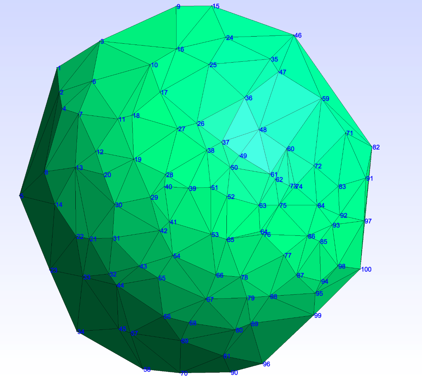
Fig. 28 Meshing produced from a thinned set of geostationary brightnessTemperature observations. See figure below for the spatial locations of the observations

The result of the application of the operator to a single observation (but with the mesh produced from the full set of observations shown in figure below) is shown below:

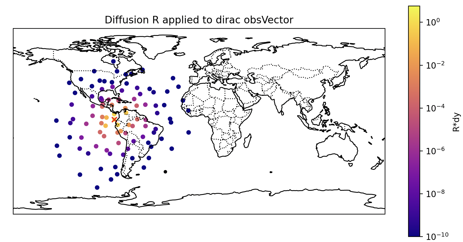
Fig. 29 The result of the diffusion operator being applied to a ‘dirac’ obsVector (a vector of all zero except for a single one) using the mesh from above.

Control Grid

In regions of sparse or irregular observations, Delaunay triangulation can produce unrealistically long-range connections between distant observation locations, leading to unphysical correlations in the diffusion operator.

An optional control grid can be added as scaffolding to guide the triangulation. A regular lon/lat grid is constructed at the specified resolution and any control grid points falling within a specified distance of an observation location are removed. The remaining control points are merged with the observation locations before mesh construction. Control grid points are assigned zero lengthscale so they guide the triangulation only and do not contribute to the diffusion.

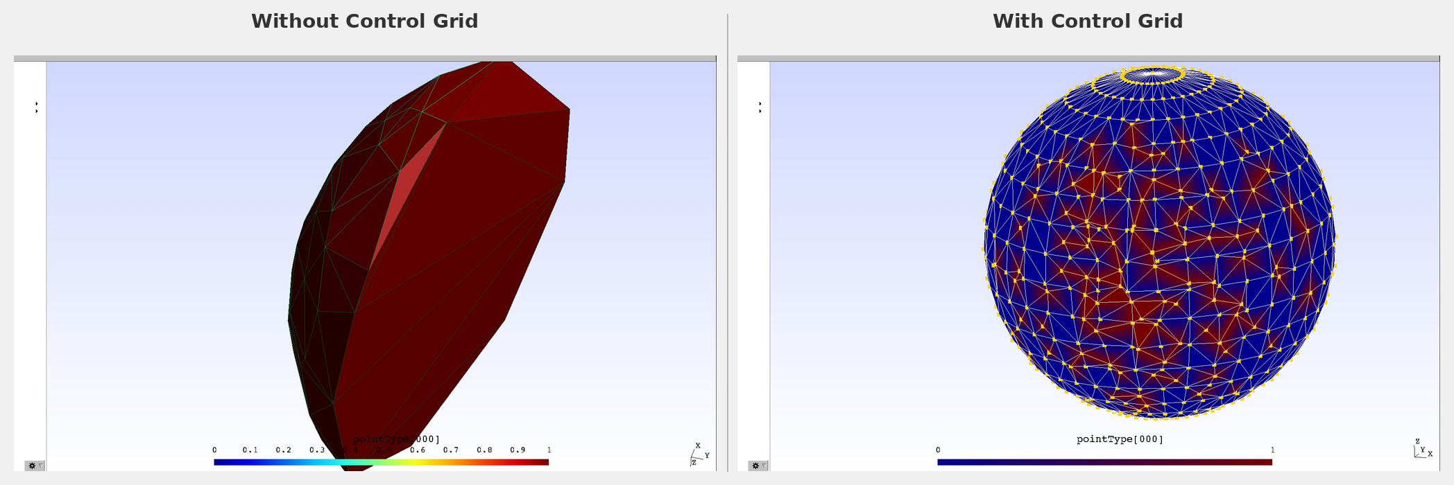
Fig. 30 Comparison of mesh without (left) and with (right) control grid for geostationary observations. Blue points indicate control grid points, red points indicate observation locations. The control grid eliminates the unrealistically long-range connections at the edges of the observation domain.

Note

For closely-spaced observations such as aircraft tracks, the control grid alone is not sufficient. Very small inter-observation distances cause the number of horizontal diffusion iterations to become very large. Gaussian thinning is recommended before applying this operator to such observation types.

Parallelization (MPI distribution requirements)

The operator runs on any number of PEs, and the result does not depend on the PE count. Two requirements are placed on the observation distribution when running on more than one PE:

• it must be non-overlapping (each observation owned by exactly one rank) — overlapping distributions such as Halo or InefficientDistribution are rejected with an error;

• it must be geographically contiguous (each rank owns a single connected region of observations). This cannot be detected at runtime: a non-contiguous distribution such as RoundRobin will run without error but produce incorrect correlations.

In practice the Atlas distribution satisfies both requirements.

obs space:
  distribution:
    name: Atlas
    grid:
      type: regular_lonlat
      nx: 72
      ny: 36
      partitioner: equal_regions

If running on more than 1 PE, the code will check that the Atlas distribution is being used. To use a non-Atlas but still geographically contiguous distribution allow any distribution: true should be included in the yaml configuration. Setting allow any distribution: true with a non-geographically contiguous obs distribution is undefined behavior, so please do not do this.

For regional observation sets, such as a geostationary satellite’s disk, a global distribution grid wastes ranks: partitions falling outside the observed region own no observations. Use a regional atlas grid covering the observation domain instead, so the partitions (and therefore the observations) are spread across all PEs. For example, for a GOES-East disk:

obs space:
  distribution:
    name: Atlas
    grid:
      type: regional
      nx: 36
      ny: 36
      north: 80
      south: -80
      east: 10
      west: -160
      partitioner: equal_regions

Note

The regional domain must contain every observation location; an observation falling outside the grid cannot be assigned to a partition and atlas will abort (Could not find point ... in "nearest" polygons). Ranks owning zero observations are otherwise harmless — the result is identical, just with idle PEs.

Options

The options for the operator include:

• correlation variable names: the names of variables to which the operator will be applied. Currently, this operator is only supported for use with a single variable.

• correlation lengthscale: correlation length scale in meters, interpreted by default as a Gaspari-Cohn cutoff radius (the distance at which the compactly-supported correlation reaches zero). Internally it is converted to the Daley length expected by oops::Diffusion (a factor of 1/3.67), the same convention used by the SABER Explicit Diffusion block. See as gaussian to change this interpretation.

• as gaussian (default: false): if true, correlation lengthscale is instead passed through unchanged as the Daley length (the standard deviation of the Gaussian profile the operator emulates).

• diagonal loading (default: 0.1): nugget fraction \(\alpha \in [0, 1]\) blending a diagonal (uncorrelated) component into R: \(R = (1-\alpha) D^{1/2} C D^{1/2} + \alpha D\). The diagonal of R equals the prescribed error variances for any \(\alpha\); values greater than zero bound the smallest eigenvalue of R away from zero, which substantially speeds the iterative (GMRESR) \(R^{-1}\) solve when the correlation length is large relative to the observation spacing. Set to 0.0 for a pure correlated R.

• Number of iterations for computing the inverse (default: 100): maximum number of GMRESR iterations used for the iterative \(R^{-1}\) solve.

• Accuracy of inverse (default: 1.0e-7): convergence tolerance of the GMRESR \(R^{-1}\) solve.

• normalization iterations: number of iterations used to calculate the set of grid-dependent normalization coefficients. See the documentation of the SABER Explicit Diffusion block for more details on the normalization procedure. For an operational/scientifically valid situation a value of at least ~10000 is recommended.

• output diffusion mesh (default: false): write the diffusion mesh to a gmsh file (filename will be diffusion_mesh.msh).

• control grid (optional): parameters for the optional control grid:

  • grid spacing in degrees: resolution of the control grid in degrees. Choose this carefully based on obs network geometry to avoid unwanted connections

  • remove within meters: distance threshold in meters. Control grid points within this distance of any observation location are removed.

Below is an example of a YAML configuration of the diffusion-based R operator with a control grid:

obs error:
  covariance model: diffusion
  correlation variable names: [brightnessTemperature]
  obs channels: [11]  #redundant with channels in obsSpace parameters
  correlation lengthscale: 200000. # meters, Gaspari-Cohn cutoff (see `as gaussian`)
  normalization iterations: 10000
  output diffusion mesh: true      # if not present will default to false
  control grid:
    grid spacing in degrees: 5
    remove within meters: 50000