SABER User Guide (B-Matrix How-Tos)
Within the JEDI system, a SABER B-Matrix (composed of one or more SABER block-chains)
can be encapsulated in an oops::ErrorCovariance or natively within a
saber::ErrorCovariance. If all the components of the B-Matrix are SABER
block-chains, using the native saber::ErrorCovariance is recommended:
background error:
  covariance model: SABER
SABER block-chains enable many advanced techniques for modeling multi-variate and length-scale aware correlations and localization. The vocabulary and language for describing these techniques with SABER are unique and idiosyncratic. Some of the techniques described here may or may not go by other names in other B matrix models, so the specifics of the techniques to which these terms refer and how they are configured are described in detail here.
Multivariate Strategies
The options for enabling different cross-variable correlation schemes (including what is sometimes
called Variable Dependent Localization or VDL) in SABER are chosen by setting a multivariate strategy.
There are 4 multivariate strategy options: univariate, duplicated,
duplicated and weighted, and crossed. These strategy were initially only implemented
at the individual SABER block level (e.g., for the BUMP-based and FastLAM blocks), but now they are
also implemented at a higher Saber Central Block level allowing the options/strategies to be used
with blocks for which the strategies had not been explicitly implemented before.
For both block-specific and higher implementations, the main idea is to collect sets of variables
into groups for which different covariance parameters (like length-scales) will be applied.
The multivariate strategy determines how correlations are handled between variables
within and across groups.
WARNING: the yaml configuration required to set up variable groupings at the saber block level differ from block to block.
The documentation in this section is largely a re-iteration of parts of this document: Multivariate localization
The mathematical descriptions of each of the multivariate strategy options consider an increment
\(\delta \overline{\mathbf{x}}\) with five variables separated into 2 groups (though an
arbitrary number of groups is supported):
where the first index indicates a different physical variable (e.g. \(\mathbf{x}_{1,1}\)
is air temperature, and \(\mathbf{x}_{4,2}\) is the surface pressure) and the second index
indicates to which group the variable belongs. (FYI: some blocks allow variables within
the same group to have different numbers of vertical levels.)
Let’s consider a localization operator \(\mathbf{L}\) which can be factored into the form:
The following strategies/options determine how two different localization (and correlation) operators
(or the same operator but with different fit/calibration parameters) for the different variable
groups will be applied within and across the groups. This typically occurs if there are different
localization length scales associated with the two (or more) different groups requiring differently
calibrated localization operators.
For each different strategy, the details of the operation resulting in an increment \(\delta \mathbf{x}\):
with a \(\delta \overline{\mathbf{x}}\) (representing an update coming from a processed observation) composed of the two groups of variables with a \(\mathbf{L}_1 = \mathbf{U}_1 \mathbf{U}_1^T\) tuned for the variables in the first group of variables and a \(\mathbf{L}_2 = \mathbf{U}_2 \mathbf{U}_2^T\) tuned for the second group of variables will be described.
Note
Although (for consistency) an ensemble localization operator \(\mathbf{L}\) was chosen
in the equations above, the multivariate strategy options also apply to correlation
operators used in parametric/static covariance models. For the parametric/static covariance
case, all the \(\mathbf{L}\)’s on in this section can be replaced with \(\mathbf{B}\)’s
(and a replacement of \(\mathbf{L} \circ \mathbf{B}_{ens}\) with \(\mathbf{B}\) in
(50)). Though, for the correlation operator in a parametric/static covariance,
typically only the univariate option is used.
In all the examples below, the \(\mathbf{L}\) operator will be a single SABER central block.
The univariate strategy
This is the simplest strategy, and it will effectively result in no cross-correlations between any variables. This options is typically used in a central block for a static covariance, where we have transformed into a control vector space where correlations between the central block variables are (ideally) zero. Mathematically the expanded \(\mathbf{L}\) will take the form:
For a specific example, consider the application of \(\delta \mathbf{x} = \mathbf{B} \delta \overline{\mathbf{x}}\) in a Dirac test where, \(\delta \overline{\mathbf{x}}\) is all zeros EXCEPT for a single value of one in the variable \(\mathbf{x}_{4,2}\):
Each of the five elements in the vector above is also a vector, and the vector notation has been selectively dropped for ease of formatting (moving forward all vector notation will be dropped).
The resulting increment, \(\delta \mathbf{x}\), will ONLY have non-zero values in locations representing the \(\delta \mathbf{x}_{4,2}\) variable. The increment for all other variable (e.g. \(\delta \mathbf{x}_{1,1}\) and \(\delta \mathbf{x}_{5,2}\)) will be zero. That is, \(\delta \mathbf{x}\) will have the form:
This may not seem like a particularly useful case, but when used in a static covariance, the outer vertical balance operator blocks in the block-chain will be responsible for spreading/transforming this univariate increment into the other variables.
The duplicated strategy
The duplicated strategy will enable correlations only between variables within the same
group, so variables in separate groups will still be non-correlated.
Mathematically, the \(\mathbf{L}\) operator takes the form:
In this case, the same dirac input vector \(\delta \overline{\mathbf{x}}\) with a single value of one in variable \(\mathbf{x}_{4,2}\) will produce an increment \(\delta \mathbf{x}\) of the form:
The duplicated and weighted strategy
The duplicated and weighted strategy is a generalization of the duplicated strategy which
allows the maximum correlation between variables within the same group to be modulated. So, for
example, this can be used to ensure that cross-variable correlations between errors in two
different variables at the same grid location have a lower magnitude than auto-correlations
(correlations between the errors in a specific variable with itself).
In this case, the mathematical form of the \(\mathbf{L}\) operator, except for the addition of extra
weight elements (\(w^g_{m,n}\) where the index \(g\) represents the variable group and the
indices \(m\) and \(n\) represent variables), is the same as for the duplicated case:
The increment \(\delta \mathbf{x}\) produced from the same dirac \(\delta \overline{\mathbf{x}}\) with a one in the \(\mathbf{x}_{4,2}\) vector will have the same form as (51). The only difference will be in the values for many of the non-zero elements.
The crossed strategy
The crossed strategy enables cross-correlations between variables in different groups, accounting
for the different correlation or localization operators for the different groups.
Mathematically, the \(\mathbf{L}\) operator with the crossed option takes the form:
In the case, the same dirac test we’ve been considering in the examples above will result in an increment \(\delta \mathbf{x}\) where all values could be non-zero:
As implied by the form of the localization in the elements of the off-diagonal (cross group) blocks in the
matrix above, the crossed option can only be used with saber central blocks that have implemented a
multiplySqrt() method.
Multi-scale Localization (MSL)
In SABER, multi-scale localization (MSL) refers to a specific application of scale-aware localization in which ensemble members (or ensemble perturbations) are filtered into separate wavebands with the localization for each waveband occuring independently. There are no cross-scale correlations with this localization technique which is an implementation of the method described by [Bue12].
To implement multi-scale localization in a dirac test or a variational application, the ensemble members (or ensemble perturbation) can first be filtered off-line using the ProcessPerts application, or filtered on-line within an ErrorCovarianceToolbox or variational application. Both on-line and off-line filtering can be applied to full ensemble members or ensemble perturbations.
In the off-line approach, sets of filtered-ensembles (one for each waveband) are written and stored
on-disc until they are read and used when applying the B-matrix, exactly like reading a non-filtered
ensemble for a standard ensemble localization. An illustration of the ProcessPerts
ensemble filtering producing two (one long scale and one short scale) filtered-ensembles is shown below:
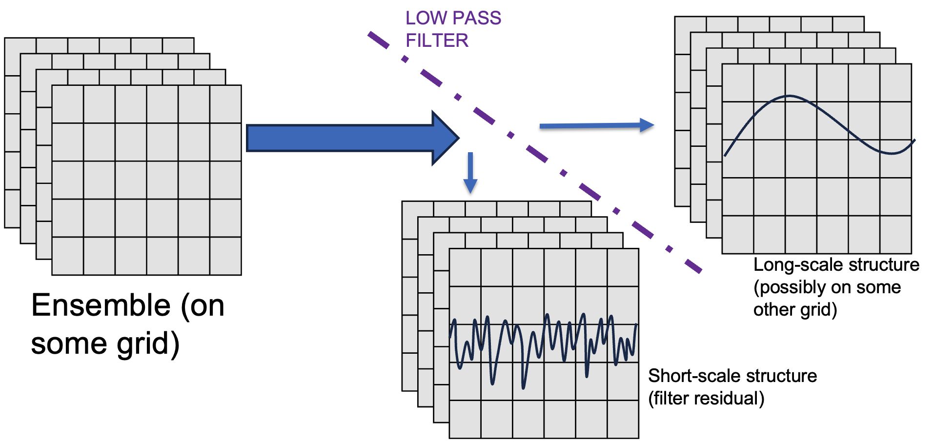
In the on-line approach filtering is applied to ensemble members via a separate OuterBlockChain
which is configured within a filter: section of an input YAML (see example in SDL
section :ref:`` for the syntax). The on-line approach saves time on file I/O and disc space
(since the filtered-ensemble members don’t have to be written to disc), but has a higher
memory requirement.
Users have many options for filtering operators. Currently the BUMP_NICAS SABER block, Explicit Diffusion, and Spectral Analytical Filter blocks can be used to filter an ensemble in to wavebands (see the ProcessPerts application documentation linked to above for more information).
To configure multi-scale localization in a saber::ErrorCovarianceToolbox or a
variational application, a hybrid covariance with each waveband making up one of the
components of the hybrid B must be used. So, either instead or in addition to the typical
Static and Ensemble components, there will be one Ensemble component per
filtered-ensemble in the full equation for B. For a case with two filtered-ensembles like the
one in the figure above plus (and optional) static component the full B will be:
where the ss and ls in the subscripts are abbreviations for ‘short-scale’ and
‘long-scale’, respectively. A SABER hybrid covariance support an arbitrary number of
components, so there is not a technical limit on the number of waveband/filtered-ensembles
used in a MSL B-matrix, but there are computational and scientific reasons to
limit the number of filtered-ensembles.
An outline of the yaml structure for this hybrid B (in which the filtered-ensembles are filtered off-line) is shown below:
background error:
  covariance model: SABER
  covariance type: hybrid
  run components recursively: true
  components:
  # Static Component
  # ================
  - covariance:
      saber central block:
        saber block name: <central block for static component>
        <central block config>
      saber outer blocks:
      - saber block name: <outer block 1 for static component>
        ...
      - saber block name: <outer block N for static component>
        ...
      ...
    weight:
      value: alpha
  # Long-scale Ensemble Component
  # =============================
  - covariance:
      covariance type: ensemble
      <ENSEMBLE CONFIG>:
        # ensemble configuration goes here:
        # including i/o config for LONG-scale filtered-ensemble
        # produced by ProcessPerts
      localization:
        saber central block:
          saber block name: <central block for LONG-scale filtered-ensemble localization>
            <central block config>
        saber outer blocks:
        - saber block name: <outer block for LONG-scale filtered-ensemble localization>
        ...
      saber outer blocks:
      - saber block name: <outer block for LONG-scale filtered-ensemble>
        ...
    weight:
      value: beta
  # Short-scale Ensemble Component
  # =============================
  - covariance:
      covariance type: ensemble
      <ENSEMBLE CONFIG>:
        # ensemble configuration goes here:
        # including i/o config for SHORT-scale filtered-ensemble
        # produced by ProcessPerts
      localization:
        saber central block:
          saber block name: <central block for short-scale filtered-ensemble localization>
            <central block config>
        saber outer blocks:
        - saber block name: <outer block for short-scale filtered-ensemble localization>
        ...
      saber outer blocks:
      - saber block name: <outer block for short-scale filtered-ensemble>
        ...
    weight:
      value: gamma
Scale Dependent Localization (SDL)
Scale Dependent Localization (SDL) is a generalization of the MSL case described above and includes cross-scale contributions to the calculation of the covariance. Representing the MSL ensemble case above as a sum over scales \(s\) (i.e. wavebands):
where \(w_s\) is taking the place of the \(\beta\) and \(\gamma\) coefficients used in the MSL equations in the previous section and \(\mathbf{B}_{s}\) is the ensemble covariance from a filtered-ensemble.
The mathematical representation of the SDL includes a second sum over the user-defined scales (also called wavebands). It also requires ‘factoring’ the localization operator and writing the mathematical representation in a form that more closely matches how the localization is implemented (see Equation (48)):
Thus, an SDL can only be setup with localization operators (Central Blocks) that implement
a multiplySqrt() method. The SDL technique (which treats cross-scale correlations
similar to the way the The crossed strategy treats correlations across variable groups)
uses an extended control vector, which increases the memory requirement for using this
technique. It is also required that the same geometry representation/grid resolution is used
for all the filtered-ensemble members across all scales. So, filtering a low waveband onto
a courser grid than higher wavebands to reduce disc space or reduce runtime when applying
the localiztion, which is an option with the MSL technique, is NOT compatible with the SDL
technique.
See below for an example YAML outline for applying SDL with on-line scale separation:
background error:
covariance model: SABER
covariance type: ensemble
recursive perturbations processing: true   # applies filtering recursively
multiscale strategy: crossed               # the `crossed` strategy includes cross-scale contributions to covariance
                                           # the default strategy, `separated`, will result in an on-line scale separation
                                           # WITHOUT cross-scale correlations (i.e. the MSL case described above)
ensemble:
  <members config>
scales:
# first low-pass filter
- filter:
  <OuterBlockChain (list of OuterBlocks) which applies first filter>
# Localization for Lowest Waveband
  localization:
    localization method: SABER
    saber central block:
      saber block name: <Central Block Name>
      ...  # central block config
      saber outer blocks:
      <list of Outer Blocks>
# second low-pass filter
- filter:
  <OuterBlockChain (list of OuterBlocks) which applies second filter>
# Localization for Middle Waveband
  localization:
    localization method: SABER
    saber central block:
      saber block name: <Central Block Name>
      ...  # central block config
      saber outer blocks:
      <list of Outer Blocks>
# Filtering recursively, so last band is residual of first two filters (no third filter)
# Localization for Highest Waveband
- localization:
          localization method: SABER
    saber central block:
      saber block name: <Central Block Name>
      ...  # central block config
      saber outer blocks:
      <list of Outer Blocks>